COMSOL Blog

Modeling of Excitations with the Magnetic Field Formulation

by Walter Frei

April 27, 2026

When using the AC/DC Module, an add-on to the COMSOL Multiphysics^® software, there are five interfaces within which we can model time-varying magnetic fields and inductive effects. Each solves a different form of Maxwell’s equations and has different modeling benefits. Here, we will look in depth at one of these interfaces, the Magnetic Field Formulation (MFH) interface, and how to use it to model inductive phenomena.

A Quick Overview of the Different Formulations

The five interfaces that can be used to solve for time-varying magnetic fields within the AC/DC Module are:

Magnetic Fields interface
Magnetic and Electric Fields interface
Magnetic Fields, Currents Only interface
Rotating Machinery, Magnetic interface
Magnetic Fields Formulation interface

The first of these, the Magnetic Fields interface, is by far the most commonly used and is the workhorse of most inductive modeling. It solves for the magnetic vector potential, the \mathbf{A}-field, and has convenient ways to excite structures such as: lumped port boundary conditions, coil domain conditions, and background field excitations. Most people do, and should, start their modeling with this interface.

Next, the Magnetic and Electric Fields interface solves for both the \mathbf{A}-field and the electric potential, the \mathbf{V}-field, making it an \mathbf{A}–\mathbf{V} formulation and introducing additional complexity. This added cost is warranted primarily in two cases:

When solving magnetohydrodynamic models
When solving at line frequencies, where you need to very precisely model the losses within dielectrics and at interfaces

The Magnetic Fields, Currents Only interface is useful strictly when there are no magnetic materials present. It is primarily meant for computing partial inductances. It also solves for the \mathbf{A}-field but does so using Lagrange elements rather than Curl elements, making it less computationally expensive.

The Rotating Machinery, Magnetic interface, as its name implies, is for modeling of motors and generators. This formulation allows parts to rotate and move relative to each other by solving for both the magnetic vector potential and the magnetic scalar potential, the V_\text{m}-field, which introduces additional cost and complexity. For an introduction, see our Motor Tutorial Series.

These formulations are all derived from Maxwell’s equations and all solve for the \mathbf{A}-field, either on its own or with an additional field. Contrast this with the Magnetic Fields Formulation interface, which is, of course, also derived from Maxwell’s equations but instead solves for the magnetic field, the \mathbf{H}-field, in the following form in the time domain:

\nabla \times \left( \frac{1}{\sigma } \nabla \times \mathbf{H} \right) = \frac{\partial \mathbf{B}}{\partial t}

and in the frequency domain:

\nabla \times \left( \left( \sigma + j \omega \epsilon_0 \epsilon_r \right)^{-1} \nabla \times \mathbf{H} \right) = j \omega \mathbf{B}

The solutions to these equations are also solutions to Maxwell’s equations, so why would we use this instead of the \mathbf{A}-field formulations? There are (at least) two reasons:

When dealing with nonlinear materials, it is possible to introduce specific types of nonlinearities with respect to currents that arise in superconductors, as well as admitting simpler ways of entering nonlinearities with respect to the magnetic field.
The \mathbf{H}-field formulation admits different ways of exciting the system. Depending upon your modeling needs, these can simplify the model setup.

It is this second point that we will examine in more detail here within the context of frequency-domain modeling. Most of the frequency-domain excitations that we will introduce will also work in the time domain, with a few exceptions that will be explicitly addressed.

Understanding the Common Boundary Conditions

The Magnetic Field Formulation interface, or the \mathbf{H}-field interface, includes four boundary conditions that are in common with the \mathbf{A}-field formulations and have the same interpretations:

Magnetic Insulation boundary condition: This is primarily interpreted as a boundary to a perfectly conductive material. For a discussion about the various other ways in which this condition can be interpreted, see our Learning Center article: “Understanding the Magnetic Insulation Boundary Condition”.
Perfect Magnetic Conductor boundary condition: This condition is primarily interpreted either as a boundary to a nonconductive media or as a type of symmetry condition. For more details, see our blog post: “Exploiting Symmetry to Simplify Magnetic Field Modeling”.
Periodic boundary condition: This condition imposes periodicity, such as for structures with a twist (like submarine cables).
Impedance boundary condition: This condition models the presence of a lossy material adjacent to the modeled space. It is a frequency-domain condition and should only be used when the skin depth is much smaller than the part size. For more details, see section 4 of our Learning Center article: “Understanding the Options for Meshing and Geometric Modeling of Conductors in Electromagnetic Fields”.

These conditions do not, on their own, introduce excitations, but they can form part of the solenoidal current path that is necessary to set up a solvable model. That is, even though they do not excite a current, they can define a path along which current can flow.

Understanding the Excitation Boundary Conditions Specific to the MFH Interface

The three boundary conditions unique to the MFH interface that can be used to introduce excitations are:

Tangential Magnetic Field boundary condition: This imposes the nonhomogeneous Dirichlet condition.
Tangential Electric Field boundary condition: This introduces a nonhomogeneous Neumann condition.
Surface Magnetic Current Density boundary condition: This is also a nonhomogeneous Neumann condition but can introduce a jump in the electric field across an interior boundary within the model space.

As their names imply, these conditions involve the tangential components of the fields on the boundaries where they are applied. If you were to enter a field that is purely normal to the boundary, that would be the same as a zero contribution. That is, the Tangential Magnetic Field boundary condition with a zero tangential component would be equivalent to the Perfect Magnetic Conductor boundary condition, and the Tangential Electric Field boundary condition without a tangential component would reduce to the Magnetic Insulation boundary condition. These conditions can only excite the system if either the electric or magnetic field has a component tangential to the boundary.

To help build up our understanding of these excitations, we will be using a model of a coaxial cable. It is worth remarking that despite its apparent simplicity, the coaxial cable is probably one of the best ways of learning electromagnetics, especially since there exist analytic solutions for the electric field and magnetic field variation with radius:

E(r) = \frac{V_0}{\ln\left(\frac{r_{outer}}{r_{inner}}\right)r}

H(r) = \frac{I_0}{2 \pi r}

where the electric field points radially outwards, and the magnetic field circulates about the center. We’ll start by using these expressions to help excite our model and work forward from there.

Introducing an Electric Potential Difference with the Tangential Electric Field

We’ll begin by imposing an electric potential difference between the inner and outer conductors at one end of the model and short the other end. The short is imposed via the Magnetic Insulation boundary condition at the far end, and the insulating space around the exterior of the coax is modeled via the Perfect Magnetic Conductor boundary condition. To impose the electric potential difference, the Tangential Electric Field boundary condition is applied over the cross-sectional faces at one end, with the electric field being set to zero within the conductors, and the above equation is used to define the field over the annular face of the dielectric.

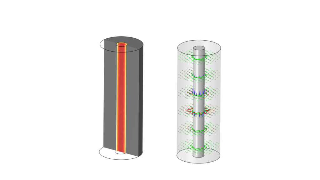
The results are shown below. Currents flow through the inner and outer conductors, and at the operating frequency, the skin depth is apparent in the plot of the losses within the volume. The arrow plots of the electric and magnetic fields and the power flow match what we should expect from a shorted section of a coaxial cable. Power flow is primarily along the axis of the cable and dissipates into heat uniformly along the length. The short at the far ends means that there are zero electric fields.

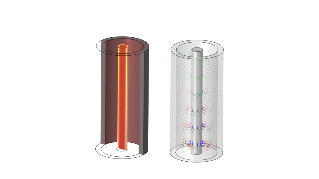Plot of the heating (left) and the electric field (red), magnetic field (green), and power flow (blue) in a coaxial cable excited with an electric field at one end and shorted at the other (right).

Note that although the losses within the dielectric are small, they are nonzero. This is because the \mathbf{H}-field formulation does require a nonzero conductivity in all domains, unless solving in the frequency domain at very high frequencies, where the displacement currents are significant. This conductivity is often referred to as a numerical stabilization term. Using a direct solver can make this stabilization conductivity quite small. We use here an expression for the electric conductivity such that the skin depth in the insulators is ~1000 times greater than the domain size. Furthermore, we do not need to use gauge fixing for models that include numerically significant inductive effects, which describes most time- and frequency-domain cases.

It is important to note that, even though a coaxial cable is a type of transmission line, there is no transmission of power through this model. The fixed electric field injects power, and this is entirely dissipated into heat within the modeled space. There is no transmission or reflection. To introduce that, we will move on to the next boundary condition type.

Using the Surface Magnetic Current Density Boundary Condition

To introduce a boundary to the nonmodeled space on either end of the coaxial cable, we need to introduce the concept of impedance — the relationship between the electric and magnetic fields. Within the coax, we know the impedance is:

Z_{coax}=\frac{Z_0}{\sqrt{\epsilon_r}}

and we can use this to define the surface magnetic current density as:

\mathbf{J}_{ms}= Z_{coax}\mathbf{H}_t

where \mathbf{H}_t is the tangential component of the \mathbf{H}-field along the boundary. This condition can be used to model an impedance on either end of the cable. We can take this one step further and introduce a source term as well:

\mathbf{J}_{ms}= Z_{coax}\mathbf{H}_t+2\left( \mathbf{n \times E}_0 \right)

The factor of two arises because the source term will excite a signal propagating into the modeling domain, as well as a signal propagating into the boundary. This factor of two assumes that the impedance of the modeled space matches the impedance of the transmission line represented by the boundary, so any mismatch of impedance will lead to some reflection. This behavior is somewhat similar to the Cable-type Lumped Port boundary condition. However, the Lumped Port boundary condition in the Magnetic Fields interface excites via a surface current, while the MFH interface excites via an electric field, so the two are not exactly analogous. Note that the Surface Magnetic Current Density boundary condition acts in contribution with other Neumann conditions, so a separate feature can be used to contribute the source term to the matched impedance term.

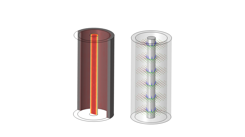Plot of the heating (left) and the electric and magnetic fields and power flow (right) in a coaxial cable excited with a matched impedance at both ends and an excitation at one end.

From the above plots, we can see that the power is flowing through the cable, so we now have a model of a two-port device. However, it is important to remark that only the frequency-domain form of the \mathbf{H}-field formulation includes the displacement current contribution. The time-domain form considers solely the inductive and conductive currents, so it is not a full-wave formulation but rather a quasi-static formulation. If you do want to model transient wave phenomena, use the Electromagnetic Waves, Transient interface, an \mathbf{A}-field formulation, as covered in the Learning Center article: “Modeling Capacitive Discharge”.

Sometimes, though, we are not interested in power flow but only the losses within the conductors. In a coaxial cable, for example, most of the losses are in the inner conductor, so we might want to analyze just that conductor and ignore the losses in the outer conductor. We also often want to assume a fixed current. For this, we use the last boundary condition, the Tangential Magnetic Field boundary condition.

Using the Tangential Magnetic Field to Impose a Current

Looking back at our analytic expressions for the magnetic field, we see that we know exactly what it will be between the inner and outer conductor, and that this expression is for the tangential component to a coaxial cylinder. With this, we can reduce our model to a cylindrical space around the inner conductor and apply the Tangential Magnetic Field boundary condition along its exterior. Conceptually, this is equivalent to imposing a tangential surface current density, so we use it in conjunction with the Magnetic Insulation boundary condition at the top and bottom to provide a solenoidal current path through the inner conductor. By imposing a magnetic field along the outside, we induce current to flow within the inner conductor. We do need to be a bit careful with this, though, as it has an interesting consequence.

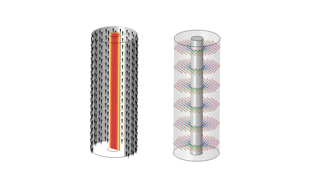
Plot of the surface currents and heating (left) and the electric and magnetic fields and power flow (right) in a coaxial cable excited with a specified tangential magnetic field along the outside. The mesh on the excitation boundary is aligned with the direction of the current flow implied by the imposed tangential magnetic field.

The magnetic field that we are applying is exact, but the finite element mesh on which it is being applied is an imperfect description of a cylinder. There can always be some geometric discretization error that leads to the modeled geometry having sharp corners and edges in the finite element space. These lead to local singularities that can lead to what looks like quite noisy fields near the boundary. We can avoid this issue by ensuring that the mesh is aligned with the direction of current flow, as shown in the image above.

There is one other feature of this method that is worth remarking on. Observe from the plot that the electric field is now aligned with the axis of the cable, rather than going between the inner and outer conductors, and that the power flow is pointing inwards towards the center. This represents a completely different kind of excitation, and it could be argued that such an excitation is not physically realizable. In terms of the current distribution, magnetic fields, and heating within the conduction, it is still a useful modeling approach.

At this point, we’ve looked at three different ways of exciting a structure. To briefly summarize:

The Tangential Electric Field boundary condition can be used to impose a potential difference between the conductors of a device.
The Surface Magnetic Current Density boundary condition can model a boundary with specified impedance along with an electric potential source term.
The Tangential Magnetic Field boundary condition can be used to impose a known current.

Although we’ve looked here at a simple geometry, exactly the same techniques can be applied on more complicated parts, as long as you keep in mind that:

The electric field should be specified at the cross section of a TEM-type transmission line or some portion of the model where it is reasonable to impose the assumption of curl-free fields.
Displacement currents are being considered in the frequency domain but not in the time domain.
The magnetic field excitation boundary has a different physical interpretation but an equivalent result in terms of the heating and requires careful meshing.

Let’s now introduce two other ways of exciting such models that are quite unique to the \mathbf{H}-field formulation.

Enforcing a Constraint on Current Within a Closed Path

One of the core capabilities of the modeling architecture of COMSOL Multiphysics^® is the ability to automatically interpret the symbolic expressions that are entered within the user interface (UI). This includes not just symbolic differentiation; it also extends to constraint elimination. Although a complete description of how this works is a bit beyond this short article, we will introduce how to implement this within the UI.

Returning to our previous model of only the inner conductor of the coaxial cable and the surrounding dielectric, we will now introduce an edge midway along the inner conductor. We want to impose the condition that a specified total current flows along the conductor, and from Ampere’s law, we know that the line integral of the magnetic field along a closed path equals the current flowing through it:

\mu_0 I = \oint \mathbf{B} \cdot d \mathbf{l}

or, for nonmagnetic materials:

I = \oint \mathbf{H} \cdot d \mathbf{l}

We can use an integration coupling to compute this current, and then use the Global Constraint feature to impose the condition that this integral must equal the desired current. From there, COMSOL^® takes care of everything else, and we can go ahead and look at the solution.

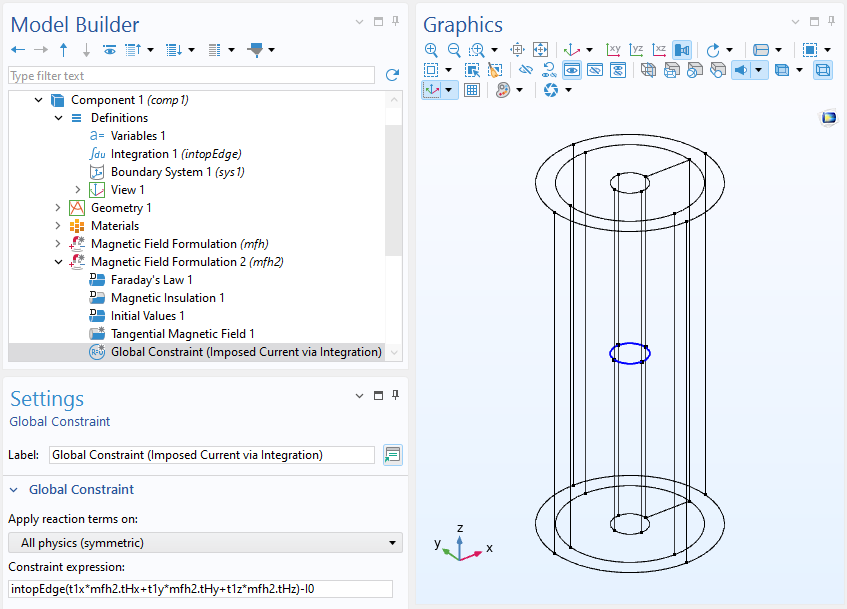Screenshot of the Global Constraint feature that enforces current flow through an integration loop over a set of edges within the Magnetic Field Formulation interface.

Plot of the heating (left) and the electric and magnetic fields and power flow (right) in a coaxial cable excited with a global constraint on the current through a loop.

Observe that the current distribution and heating profile match the previous model. The magnetic field also matches the analytic expectation. The electric field and power flow, however, should again give us pause. The power flow implies that the edge is acting as a kind of an interior line source, but this again represents something that is not physically realizable, so the electric field does not have meaning. Despite that, the current distribution and the heating from such a model can be used. Note also that the heating distribution is smooth around the excitation edge.

The advantage of this approach is that we can excite current flow through any kind of structure. We do not need to impose any excitation at the boundaries of the modeling space. That is, we can excite a conductive loop entirely within the model space or different currents in different conductors.

Coupling the Magnetic Field Formulation to the Magnetic Fields, No Currents Interface

The last type of excitation that we will cover involves using another physics interface, the Magnetic Fields, No Currents interface. This interface solves for the magnetic scalar potential, the V_\text{m}-field, and, as its name implies, is classically meant for the modeling of systems where there are no currents present.

It turns out, though, that when used in combination with the \mathbf{H}-field formulation, the V_\text{m}-field interface can introduce an excitation using the Magnetic Scalar Potential Discontinuity boundary condition. This condition has to be applied to a boundary representing the cross section of a closed loop of current. The current can flow either through the volume of a conductive domain modeled using the \mathbf{H}-field or implicitly along the Magnetic Insulation boundaries of the V_\text{m}-field interface.

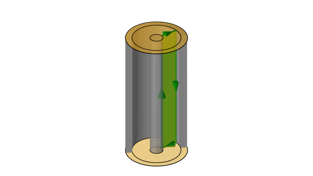Schematic of a coaxial cable excited using the \mathbf{H}–V_\text{m} approach. The Magnetic Scalar Potential Discontinuity boundary (green) excites current to flow along a solenoidal path through the two conductive domains (grey), modeled using the \mathbf{H}-field formulation, and along the Magnetic Insulation boundaries (yellow) at the top and bottom of the modeling domain. The arrows provide a visualization of this loop around the excitation boundary.

The \mathbf{H}–V_\text{m} formulation will have less degrees of freedom (DOFs) than the \mathbf{H}-field formulation but can have greater computational costs since the resultant system matrix is nonsymmetric and usually requires a direct solver. It is conceptually, and sometimes geometrically, complex. It has the advantage that free space regions can be modeled as having zero loss, but there is no capacitive coupling though these domains. In fact, only the magnetic field is computed in the nonconductive domains, so the electric field and, hence, power flow are not defined. Only the magnetic fields, currents, and losses within the conductor can be extracted.

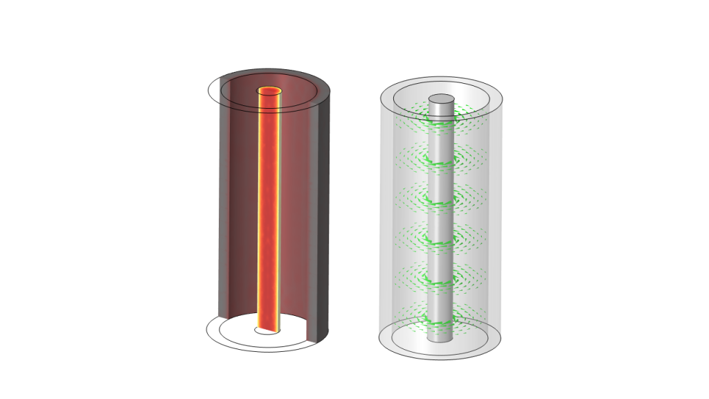Plot of the heating (left) and the magnetic field (right) in a coaxial cable modeled using the \mathbf{H}–V_\text{m} formulation.

A Quick Overview of Other Possibilities

There is a near-infinite complexity to the types of low-frequency inductive modeling that can be addressed using these excitation methods of the \mathbf{H}-field formulation. It should be emphasized that just because they can does not necessarily mean that they should be done using these approaches. It is very much something that needs to be determined on a case-by-case basis. With that being said, here are a few quick examples of other ways in which these approaches can be used.

Modeling a Unit Cell of a Twisted Cable

The Periodic Condition boundary condition can be imposed on faces that are identical but with a twist relative to each other. This boundary condition is demonstrated in the example of a twisted submarine cable and can be combined with the approach of exciting the current via a global constraint.

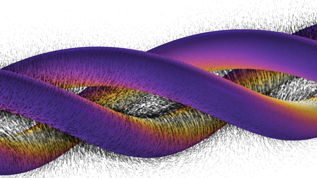A unit cell model of a one-quarter section of a twisted three-phase cable. The results on the modeled section can be patterned along the length, showing the heating and magnetic field.

Modeling a Symmetric Coil

When exploiting symmetry, it is often impractical to use the Lumped Port excitation within the Magnetic Fields interface; a Coil domain condition usually has to be used. This has a drawback at high frequencies, since the skin depth of the coil will need to be meshed very carefully. Using the MFH interface instead, the driving coil can instead be modeled using the Impedance Boundary Condition and the current imposed via the method of a global constraint.

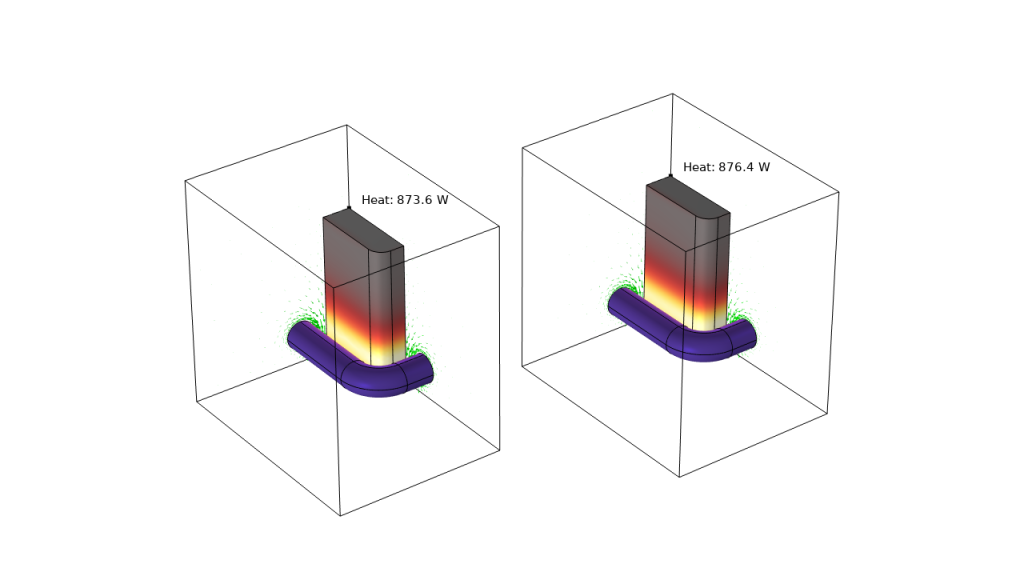A symmetric model of an inductively heated billet of material, using the \mathbf{H}-field formulation (left) and the \mathbf{A}-field formulation (right). The deposited heat is very similar.

Modeling a Solid Conductive Part within a Background AC Field

When a conductive part is exposed to an AC magnetic field, there will be induced currents within the volume of the material. As long as there are no holes in this part, which can intercept some fraction of the field, it is possible to model this using the coupled \mathbf{H}–V_\text{m} formulation. It is strictly required that the conductive material does not form a closed loop.

When using the \mathbf{H}–V_\text{m} formulation, the resultant system matrix is nonsymmetric, so computational costs will grow more rapidly than when using the \mathbf{H}-field formulation in all domains or the \mathbf{A}-field formulation, despite the lower number of DOFs. It thus is primarily useful if the ratio of the part volume to the entire modeling volume is very small.

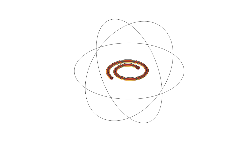A spiral piece of wire exposed to the background AC magnetic field. Note the wire does not form a closed loop. The \mathbf{H}-field is solved within the wire and excited by the boundary conditions applied to the V_\text{m}-field solved for within the surrounding space.

Closing Remarks

We have shown here a few ways in which to excite the \mathbf{H}-field formulation to solve inductive problems, and of course there are many more variations on these techniques. Although these examples all are solved in the frequency domain, they are also applicable in the time domain with the caveats noted earlier. With these examples in our toolbelt, we’re ready to further explore the electromagnetic modeling possibilities with the AC/DC Module.

Note also that many of these examples are solved using direct solvers. It is worth remarking that with the NVIDIA CUDA^® direct sparse solver (NVIDIA cuDSS), available in COMSOL^® version 6.4, one can address larger and larger problems in less time than ever before.

To gain hands-on experience with the models discussed in this blog post, click the button below.

Get the Model

NVIDIA and CUDA are trademarks and/or registered trademarks of NVIDIA Corporation in the U.S. and/or other countries.

Comments (0)

EXPLORE COMSOL BLOG