
Among the mechanisms that cell membranes exert toward homeostasis, permeability plays a central role. It regulates what can enter the cell through tiny pores in the membrane. However, in most cases permeability is limited to small target ions and molecules. To overcome this limit, electroporation is used as an artificial means to create pores in the membrane and allow for large or unrecognized molecules, such as pharmaceuticals, to enter the cell. In this blog post, we explore the key mechanisms of cell membrane electroporation.
What Is Electroporation and How Can It Be Modeled?
Biological cells feature complex self-regulating mechanisms to accomplish one goal: maintain a stable living state, in one word, homeostasis. Among these mechanisms, cell membranes’ permeability plays a central role in regulating what is allowed or not allowed to enter the cell. Simply put, cells tune membrane permeability to control the exact amount of ions, water, and nutrients upon which homeostasis is established. This control is exerted using specific membrane receptors that gate the opening state of tiny channels or pores in the membrane. An open pore allows for the passage of its target molecule across the membrane, while a closed pore blocks any passage of such a target.
The downside of such a fine regulation process is that a great number of harmless biological entities are concealed to the cell, just because they are too large or unrecognized by the cell. This is where electroporation comes to the rescue.
Electroporation, or electropermeabilization, is a technique that employs highly localized electric fields to generate pores in cell membranes, improving the cell permeability for ions, DNA, and pharmaceuticals. Electric fields cause local rearrangements of the membrane and eventually lead to the generation of pores. The electroporation process can be reversible or irreversible depending on electric field intensity and duration. In the former case, small and temporarily stable pores are created, which naturally reseal after the electric field is removed. In the latter case, pores keep expanding until they locally break the membrane, leading to the death of the cell.
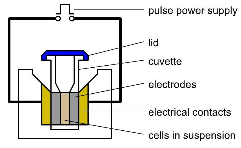 A diagram of the main components of an electroporator with cuvette loaded. Licensed under CC BY-SA 3.0 via Wikimedia Commons.
Short electroporation pulses have gained interest due to the reversibility, hence the repeatability of the electroporation process. High-intensity, nanosecond-short electric pulses have been shown capable of generating nanometric pores in cell membranes with minimal side effects for the cell. At this time scale, which is comparable with the relaxation times of cell membranes, another relevant phenomenon is considered: the dielectric dispersion of the membrane, which contributes to improving the efficacy of electroporation. Dielectric dispersion makes the dielectric properties frequency dependent. In particular, the dielectric constant decreases as the frequency increases.
Modeling Electroporation in COMSOL Multiphysics®
Based on the strong analogy between ions in a biological electrolyte and electrons in a conductor, we can treat neutral, monovalent electrolyte solutions as ohmic conductors. Under this approximation, we can resort to an equivalent electrical description of an electrolyte where the electric conductivity is proportional to the ion concentration, valence, and mobility. The electrical permittivity is that of water.
A similar analogy holds for insulating materials. In fact, the cell membrane should be considered from an electrical perspective, as a static insulating layer with a finite dielectric constant and extremely low conductivity or permeability. This is true for the cell membrane at equilibrium, but during an electroporation event, the membrane conductivity increases. Electroporated membranes no longer behave as pure static insulators, since a finite conductive path develops across them. This explains why the exchange of information between the two sides of the cell is facilitated after electroporation.
Bearing this concept in mind, the electroporation effect on cell membranes can be included by considering two conductivities: an always present static membrane conductivity, and a time-varying membrane conductivity that appears only in conjunction with electroporation. Literature models use analytical formulations for the latter conductivity.
In our tutorial model, we use the following physics-based analytical formulation, whose parameter values are taken from Ref. 1:
where N(t,V_m(t)) is the time- and membrane voltage-dependent pore density generation, \sigma_p is the pore conductivity, r_p is the pore radius, and K is a term proportional to the entrance length and energy barrier of the pore.
The adopted electrical description also benefits from its suitability for frequency-domain studies. This aspect facilitates the incorporation of the dielectric dispersion properties for the materials. We use a Multipole Debye dispersion model, owing to the availability of tabulated measurement data for the membrane and the electrolyte, and because it is compatible with both static, time-dependent, and frequency-domain analyses.
It reads:
where \varepsilon_r(f) is the frequency-dependent relative permittivity, \varepsilon_{\infty} is the relative permittivity at the high-frequency limit, \Delta \varepsilon_{\text{r} m} is the mth relative permittivity contribution, \tau_{vm} is the relaxation time corresponding to the mth relative permittivity contribution, and N is the number of poles.
These dispersive material quantities are taken from Ref. 2–3. Figure 1 shows the conductivity and relative permittivity spectrum for the intracellular and extracellular solutions, as well as for the pristine membrane materials.
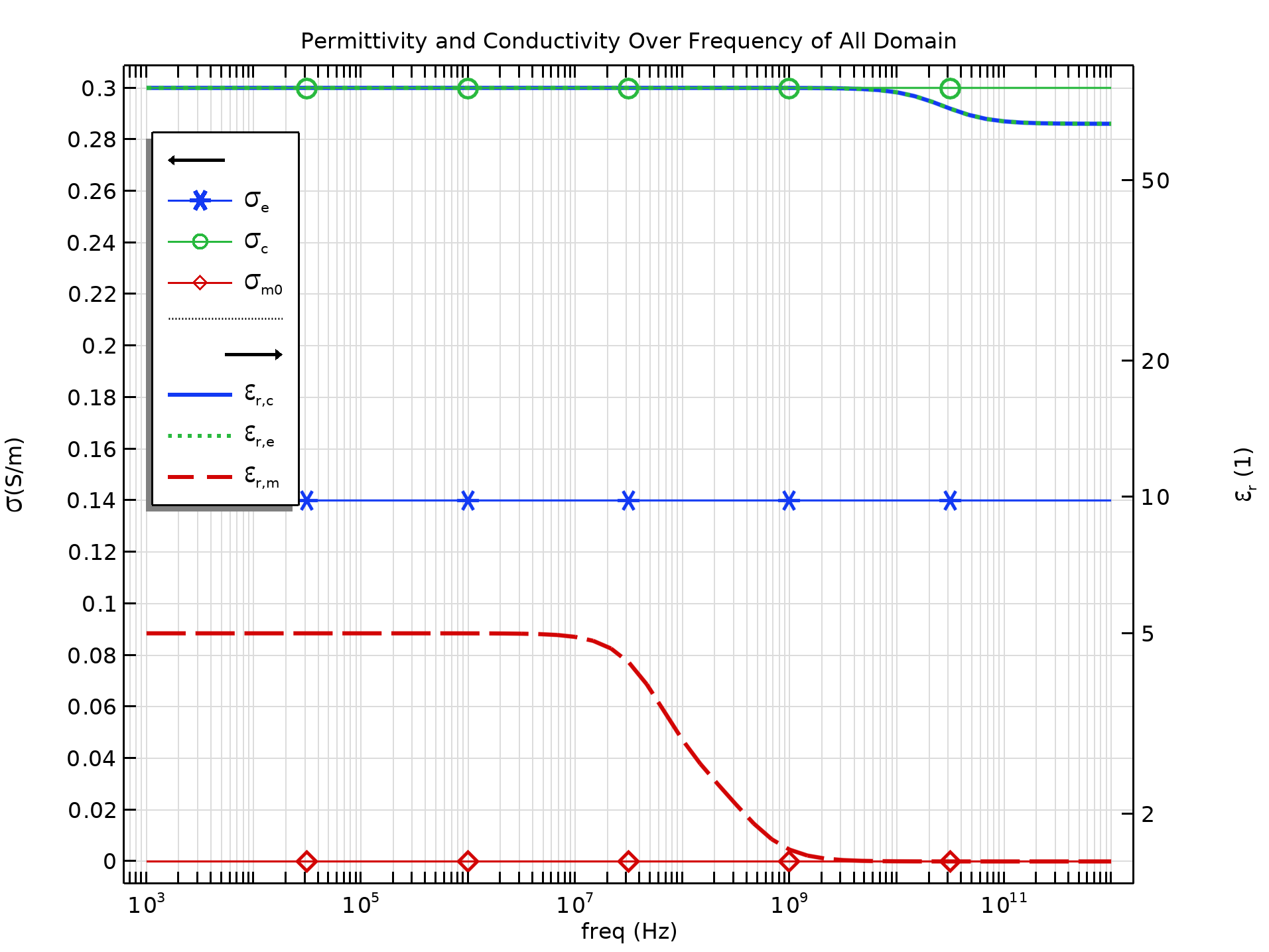 Figure 1. Conductivity and relative permittivity for the intracellular solution, extracellular solution, and pristine membrane materials, with quantities taken from existing literature.
In the COMSOL Multiphysics® software, implementing the Multipole Debye dispersive material model requires a small number of settings, as shown.
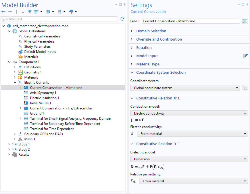
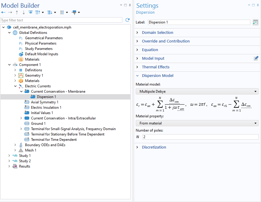
Settings for the Current Conservation node used to model the cell membrane (left). Settings for the Dispersion node (right).
Simulation Results
Now let’s look at the simulation results. In this section, the transmembrane voltage, pore density, and membrane conductivity are shown both in the frequency domain and time domain. First, we will consider two results concerning the frequency response of the system to a 10 V AC perturbation between 1 kHz and 1 GHz. Then, we display a series of results from the transient response of the system to a 650 V Gaussian pulse centered in t = 5 ns.
Figure 3a illustrates the 2D axisymmetric electric potential surface plots and electric field streamlines at three different frequencies. At low frequency (1000 kHz, left inset), the membrane behaves as a capacitor under DC excitation and a relatively small signal couples to the inside of the cell. At high frequency (1 GHz, right inset), the membrane behaves like a capacitor under AC excitation and the signal strongly couples to the intracellular domain. The central inset shows an intermediate condition between low and high frequencies.
Figure 3b displays the transmembrane voltage modulus and phase spectra at a point located at the top of the cell, supporting the findings of Figure 3a. As the frequency increases, more signal couples to the inside of the cell and the difference between the outside and the inside of the cell reduces. The rebound at 1 GHz is related to the dielectric dispersion of the membrane and electrolyte solutions.
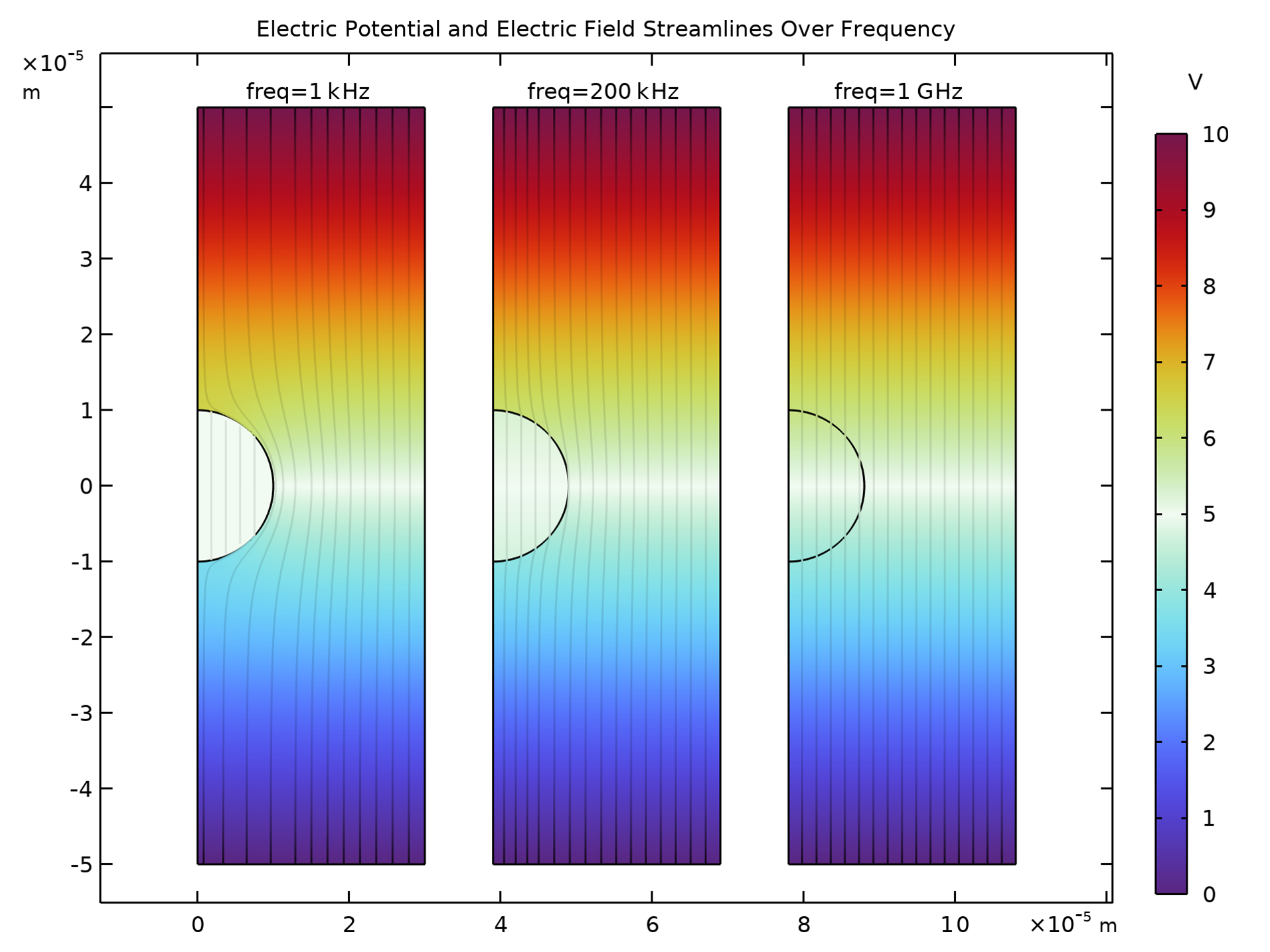
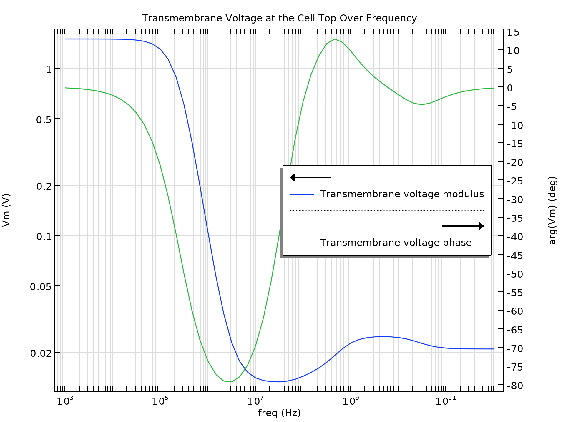
Figure 3a. Electric potential and electric field streamlines for low, intermediate, and high frequencies (left). Figure 3b. Transmembrane voltage modulus and phase spectra at the top of the cell (right).
Figure 4 depicts the same quantities as those of Figure 3b but for three time instants during the 10 ns-long Gaussian pulse centered at t = 5 ns. It confirms that a nanosecond-short pulse reproduces the qualitative behavior of a high-frequency AC excitation (Figure 3a, right inset). In addition, the solution at t = 8 ns shows that the membrane remains affected by the electroporation, as the streamlines are different than in the plot inset preceding electroporation at t = 2 ns.
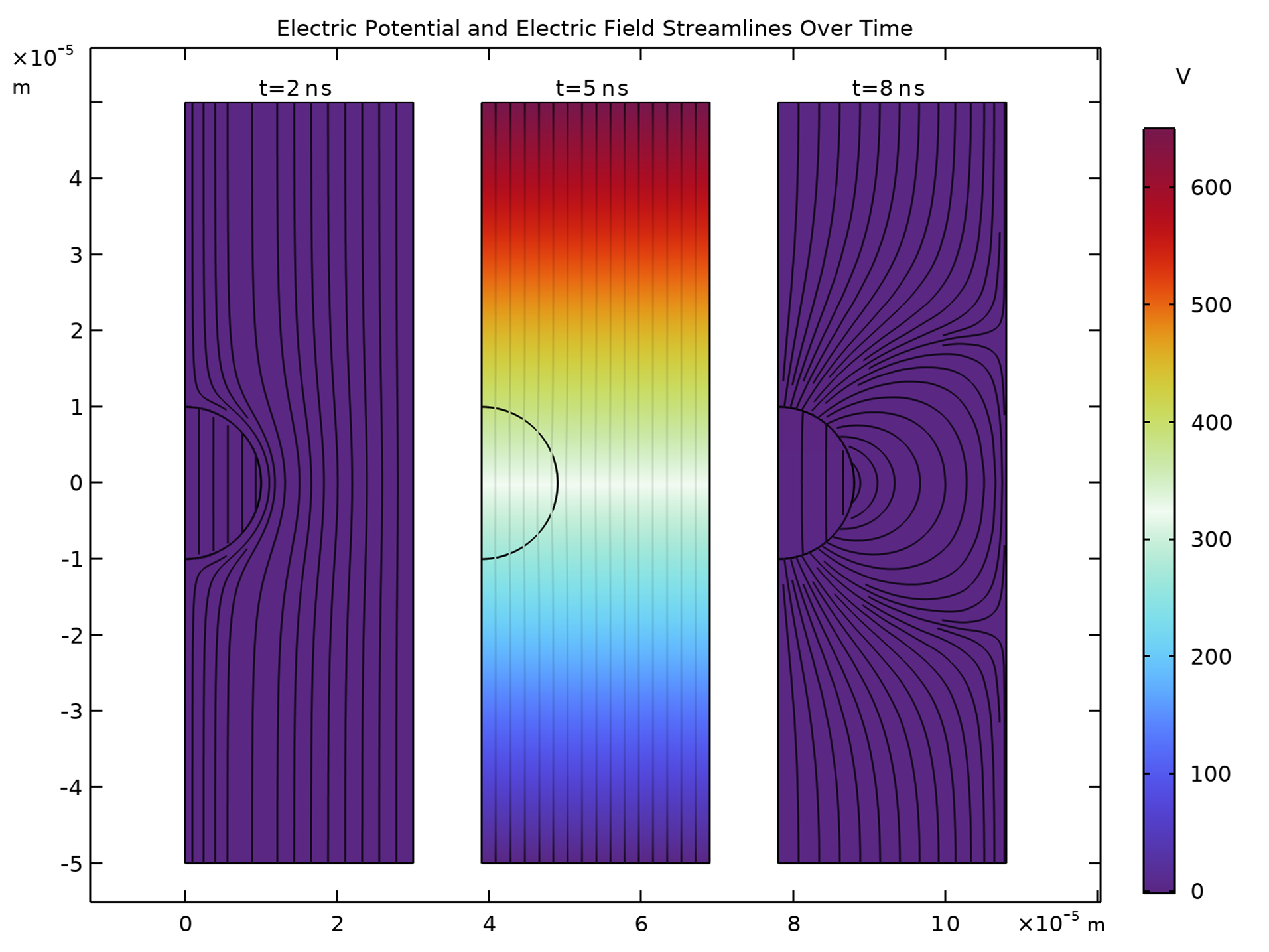 Figure 4. Transmembrane voltage modulus and phase spectra for three time instants during the Gaussian pulse.
Figure 5 shows the membrane voltage, membrane conductivity, and pore density at a point located at the top of the cell. The increase of the transmembrane voltage due to the charging of the capacitive membrane triggers an exponential increase in the pore density (right axis, log scale). This translates into a proportional increase in the membrane conductivity that in turn creates a conductive path for the potential built onto the external membrane boundary toward the intracellular domain. As a result, the transmembrane voltage gets reduced compared to the case without electroporation.
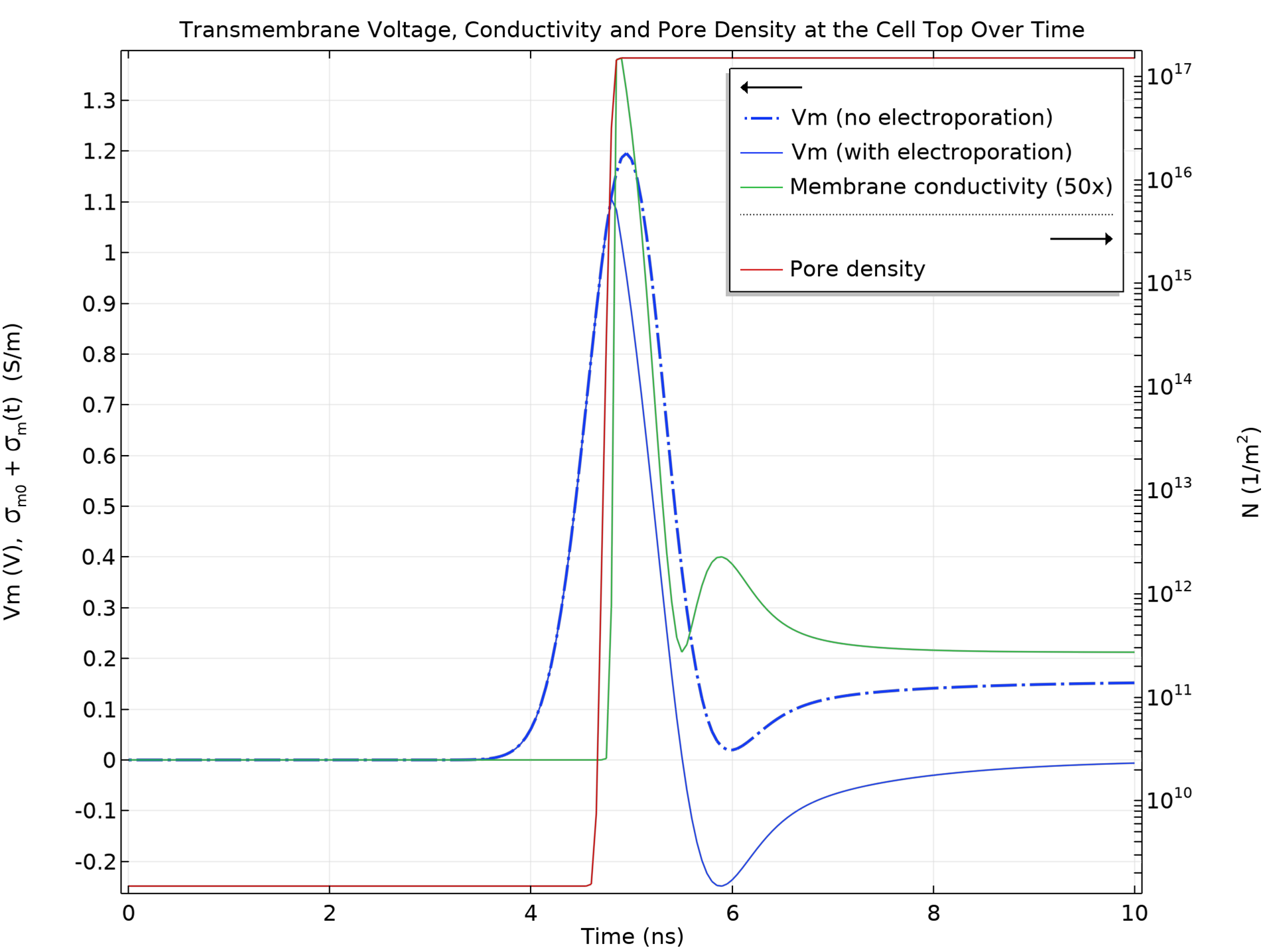 Figure 5. Membrane voltage, membrane conductivity, and pore density at the top of the cell.
Figure 6a shows the membrane conductivity along the cell’s edge at three time instants. Before 5 ns, the membrane conductivity remains close to a small static value. After 5 ns, the membrane conductivity at the cell’s poles increases significantly and remains at high values for a few more nanoseconds. Figure 6b is similar to Figure 6a but displays the transmembrane voltage. After 5 ns, the transmembrane voltage at the cell’s poles drops due to the locally increased membrane conductivity.
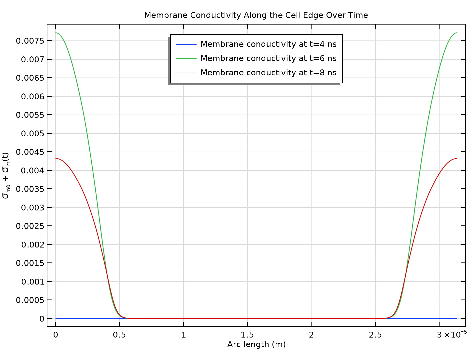
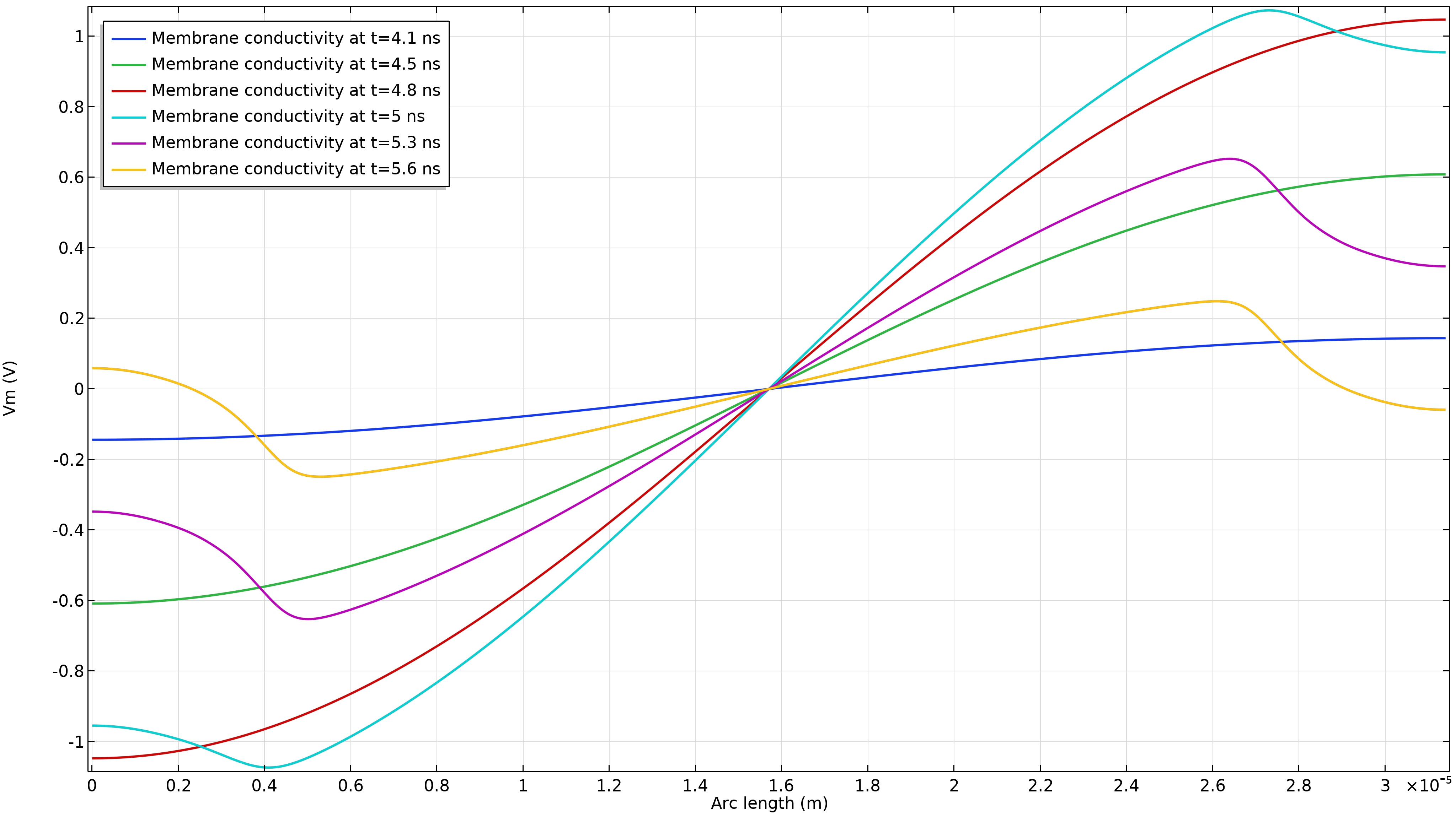
Figure 6a. Membrane conductivity at three time instants (left). Figure 6b. Transmembrane voltage at six time instants (right).
Figure 7 shows the membrane conductivity at the peak instant of the electroporation pulse.
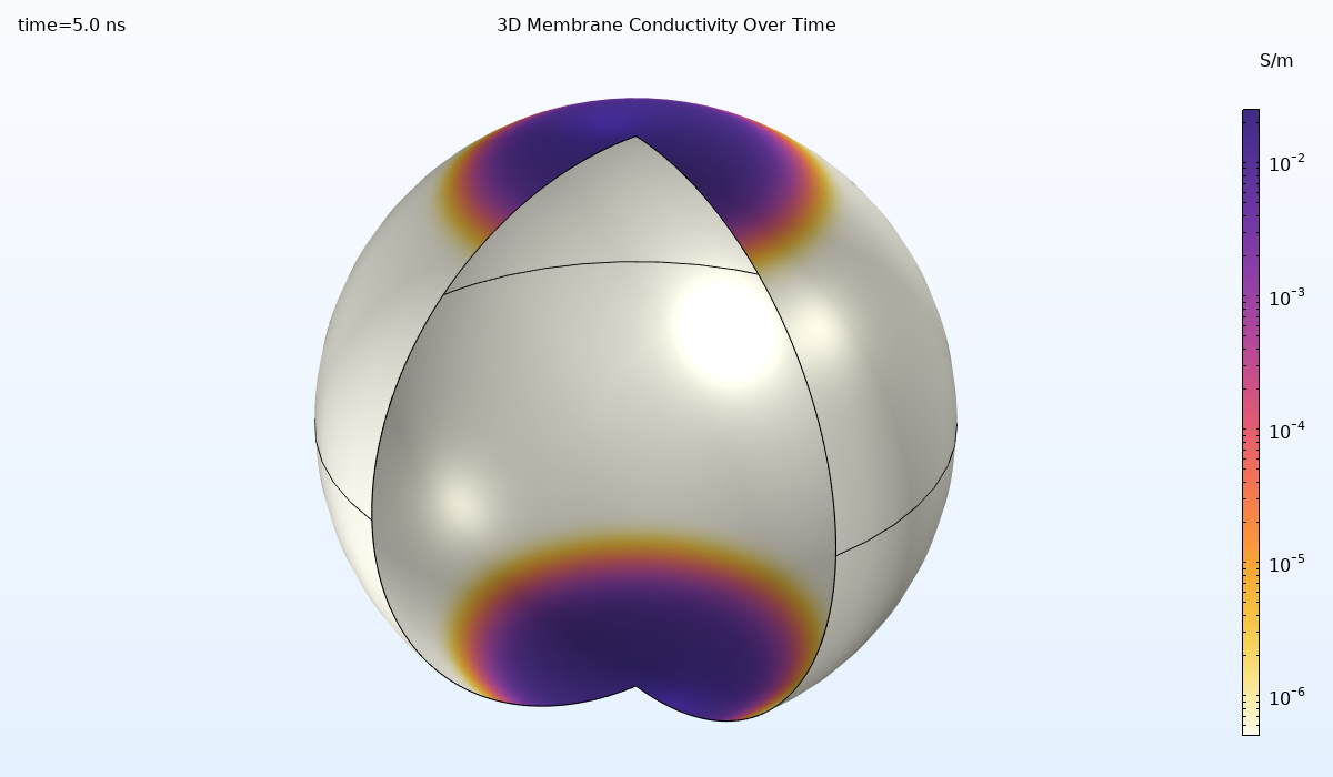 Figure 7. Membrane conductivity during peak electroporation.
The simulation results highlight that the poles are the regions mostly affected by the electroporation process.
Try It Yourself
Want to try the model featured throughout this blog post yourself? Download it via the button below, which will take you to its entry in the Application Gallery:
References
The parameter values of this tutorial model were taken from Ref. 1 with the permission of the authors’ research group (Laboratory of Biocybernetics, Department of Biomedical Engineering, Faculty of Electrical Engineering, University of Ljubljana, Slovenia), as well as from Ref. 2 and Ref. 3. The results of the present model are in agreement with those shown in Ref. 4.
- G. Pucihar, D. Miklavcic, and T. Kotnik, “A Time-Dependent Numerical Model of Transmembrane Voltage Inducement and Electroporation of Irregularly Shaped Cells,” IEEE Transactions on Biomedical Engineering, vol. 56, no. 5, pp. 1491–1501, 2009.
- R. Buchner, G.T. Hefter, and P.M. May, “Dielectric Relaxation of Aqueous NaCl Solutions,” J. Phys. Chem. A, vol. 103, no. 1, pp. 1–9, 1999.
- B. Klösgen, C. Reichle, S. Kohlsmann, and K.D. Kramer, “Dielectric Spectroscopy as a Sensor of Membrane Headgroup Mobility and Hydration,” J. Biophys, vol. 71, no. 6, pp. 325–3260, 1996.
- E. Salimi, Nanosecond Pulse Electroporation of Biological Cells: The Effect of Membrane Dielectric Relaxation, master’s thesis, Dept. Electrical and Computer Eng., Univ. Manitoba, Winnipeg, 2011.


Comments (0)