COMSOL Blog

Wave-Based Room Acoustics Modeling with Accurate Sound-Absorbing Boundary Condition

Takumi Yoshida

September 1, 2026

Properly modeling sound-absorbing boundaries is important for efficient room acoustics simulations, as discussed in Part 1 of this two-part blog series. The goal was to show the theoretical description of the local and extended reaction models and what differences appear in the random incidence absorption coefficient. As a more practical example, this blog post presents how different sound absorption models can make a difference in room acoustics with a wave-based, time-domain acoustics simulation.

Read Part 1 of this two-part blog series here.

The Importance of Acoustics in a Meeting Room

Have you ever been in a meeting where you can barely hear what the other person is saying? This is often due to excessive reverberation in the room. It is well known that a bad sound environment in the workplace can lead to poor communication, focus, and productivity. The best solution to this problem is to install acoustic absorbers, such as a suspended porous ceiling or an absorbing curtain, in a suitable place in the room. These absorbers have an air layer behind them to absorb low-frequency sound, making them highly extended reactive. It is interesting to see the difference that using different sound-absorbing boundary models makes when simulating a room with such extendedly reacting sound-absorbing functions.

Room Model and Absorption Setting

The simple room (3.5 m \times 6.8 \times 2.5 m) below was analyzed with octave bands ranging from 63 to 500 Hz (approximately 40 to 710 Hz) using the Pressure Acoustics, Time Explicit interface.

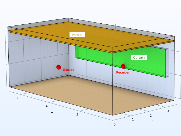A diagram showing the geometry of an analyzed meeting room.

The Gaussian pulse was applied to the source point (0.7 m, 4.15 m, 1.2 m), and at the receiver point (2.8 m, 2.35 m, 1.2 m), the pressure response was evaluated up to 0.8 s with a sampling frequency of 10000 Hz.

To solve the acoustic wave equation in the time domain, the Pressure Acoustics, Time Explicit interface uses the discontinuous Galerkin finite element method (dG-FEM), which is a memory-efficient and scalable method. The room model has typical sound absorption functions, i.e., the suspended porous ceiling and the curtain. In this blog post, these absorbers are modeled using both locally and extendedly reacting models, and the resulting differences are examined. The image above is for the extended reaction model, which includes the thickness of the porous material and the air space behind the absorbing materials. In the case of the local reaction model, the thickness and air space are not modeled explicitly, while the surface impedance at normal incident condition is assigned to the surface boundaries of the materials. The surface impedances of those sound absorbers were evaluated with submodels in the frequency domain, assuming a two-dimensional periodic structure.

The suspended ceiling is made of a 50 mm porous material. The air space behind the porous material is 180 mm and was made to absorb low-frequency sound. Since the thickness of the porous layer is large, an equivalent fluid model is used to model the ceiling absorber, including the extended reaction. The Johnson–Champoux–Allard (JCA) model is used to model the fluid property in the porous material. With this model, the complex effective density and bulk modulus of the porous material are expressed as follows:

\rho_{\rm c}=\frac{\tau_{\infty}\rho_{\rm f}}{\epsilon_{\rm p}}\left(1+\frac{R_{\rm f}\epsilon_{\rm p}}{i\omega\rho_{\rm f}\tau_{\infty}}\sqrt{1+\frac{4i\omega\tau_\infty^2\mu\rho_{\rm f}} {R_{\rm f}^2L_{\rm V}^2\epsilon_{\rm p}^2}} \right)

K_{\rm c}=\frac{\gamma p_{\rm A}}{\epsilon_{\rm p}}\left(\gamma – (\gamma-1)\left[1+\frac{8\mu}{i\omega L_{\rm th}^2P_{\rm r}\rho_{\rm f}}\sqrt{1+\frac{i\omega L_{\rm th}^2P_{\rm r}\rho_{\rm f}}{16\mu}}\right]^{-1} \right)^{-1}

Therein, p_{\rm A}, \rho_{\rm f}, \gamma and \muare respectively the absolute pressure, the density, the ratio of specific heats, and the dynamic viscosity of the fluid in the porous material. \epsilon_{\rm p}, R_{\rm f}, L_{\rm v}, L_{\rm th} and \tau_{\infty} represent the porosity, the flow resistivity, the viscous characteristic length, the thermal characteristic length, and the tortuosity factor of the porous material. \omega is the angular frequency. The table below summarizes the parameters of the porous material used in the example model.

Parameter (Unit)	\epsilon_{\rm p}(1)	R_{\rm f} (Pa·s/m²)	L_{\rm v} (mm)	L_{\rm th} (mm)	\tau_{\infty} (1)
Value	0.99	17000	0.14	0.15	1.01

Porous matrix properties used in the example model. These values are from Ref. 1.

The Poroacoustics feature, available in the Pressure Acoustics, Time Explicit interface, can be used to model the porous layer based on the equivalent fluid model. The Porous Absorber with Local and Extended Reacting Approximations for Time-Domain Modeling document is a good reference for our implementation of the time-domain equivalent fluid model. To use this feature, we should prepare the frequency-dependent data of the complex effective density and compressibility (a reciprocal of the bulk modulus) of the porous material. In the example model, these properties were calculated using the same submodel used to evaluate the surface impedances for local reaction modeling. The following screenshot shows the Poroacoustics settings for the submodel.

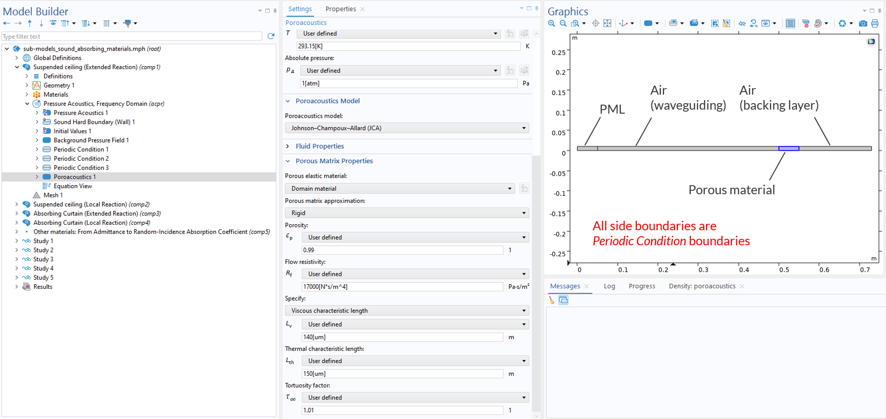Poroacoustics feature settings for submodeling of the porous material.

The following screenshots show more calculations of the material properties from the result of the submodeling.

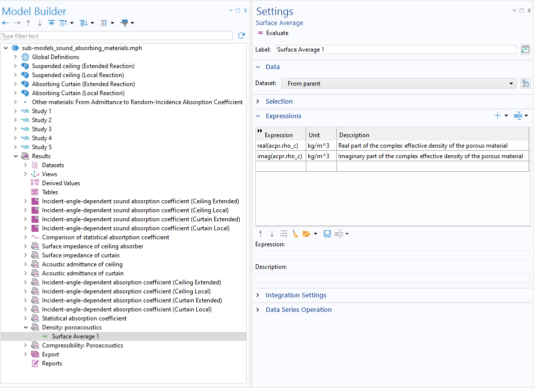
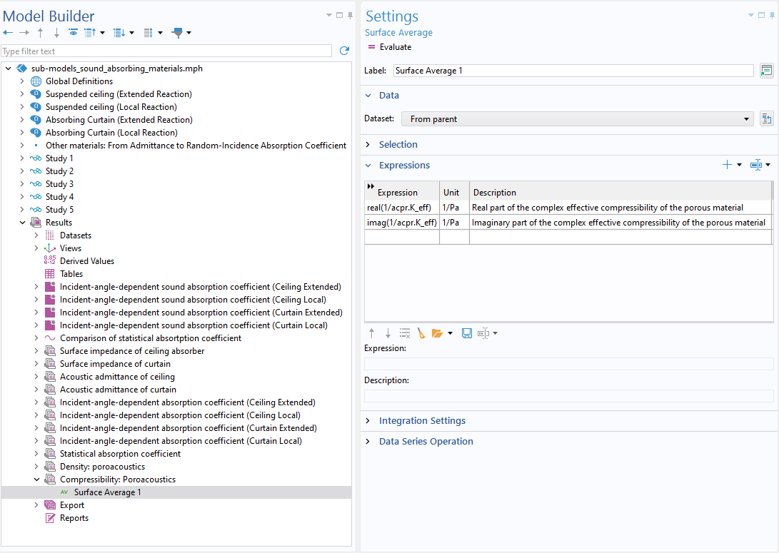
A screenshot showing the calculation of the effective density of the porous material from the 2d frequency-domain analysis.

A screenshot showing the calculation of the compressibility of the porous material from the 2d frequency-domain analysis.

Calculation of the complex effective density (left) and compressibility (right) of the porous material from the result of the 2D frequency-domain analysis.

You could also use the measured data of these material properties. Then, the frequency-dependent properties of the porous materials are imported and approximated to the rational function forms with the Partial Fraction Fit function for the analytic inverse Fourier transformation.

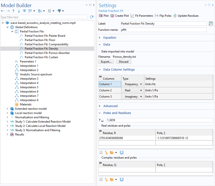
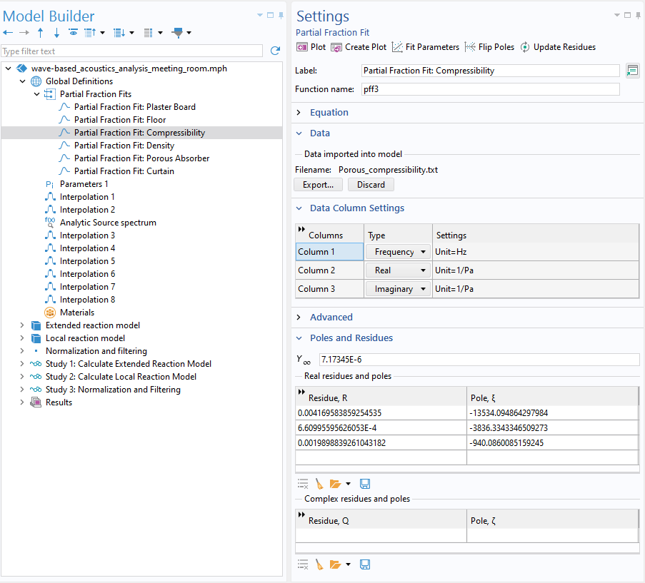
A screenshot showing how to use the Partial Fraction Fit function to approximate complex effective density of a porous material.

A screenshot showing how to use the Partial Fraction Fit function to approximate compressibility of a porous material.

Use of the Partial Fraction Fit function to approximate the complex effective density (left) and compressibility (right) to the rational function forms.

The fitted results are further imported in the Poroacoustics feature in the Pressure Acoustics, Time Explicit interface.

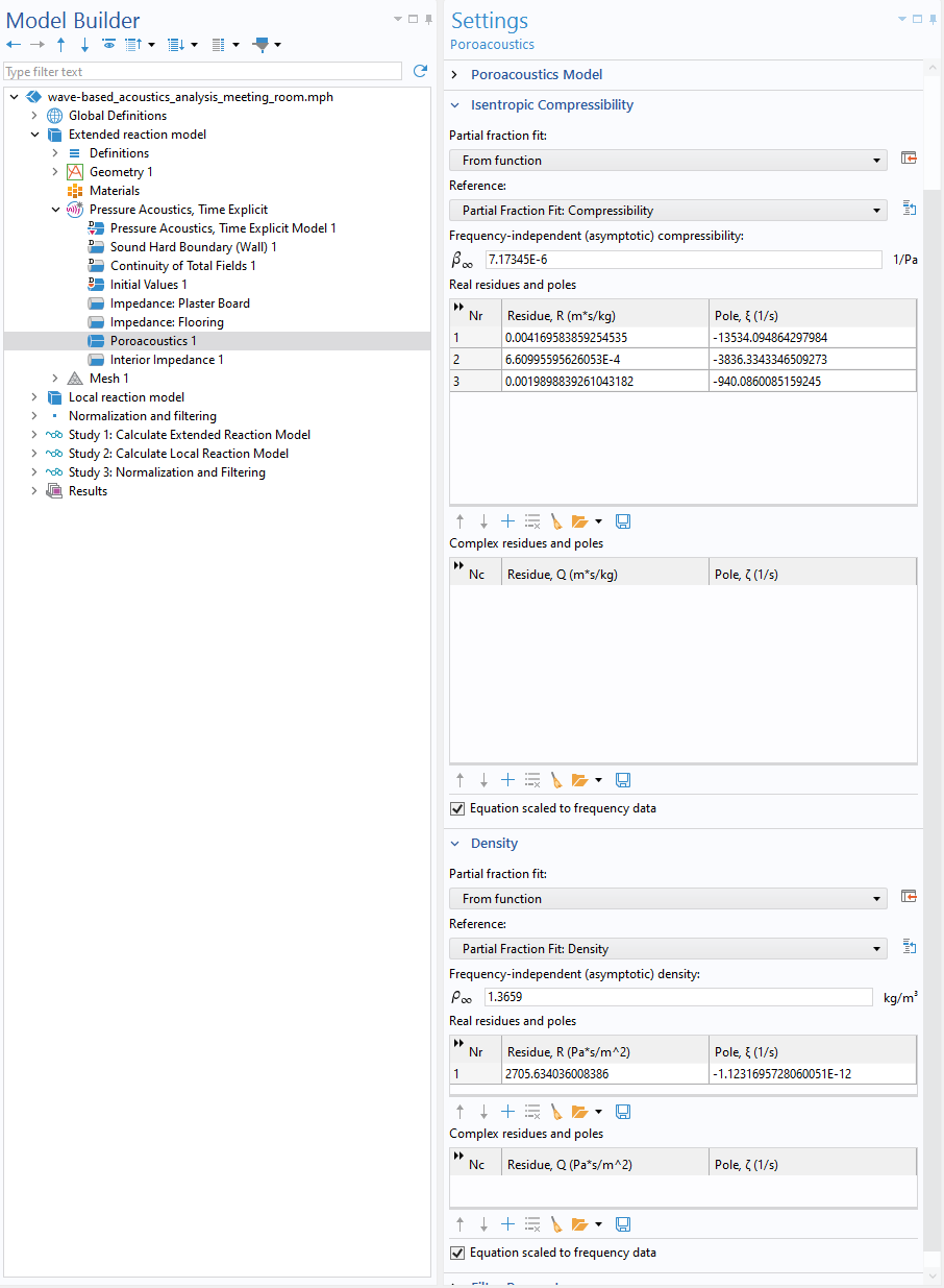
A screenshot of the Poroacoustics feature in the Pressure Acoustics, Time Excplicit interface in COMSOL Multiphysics.

Poroacoustics feature in the Pressure Acoustics, Time Explicit interface.

On the other hand, the extended reacting absorbing curtain was modeled using a transfer impedance, on the assumption that it was very thin. We assumed that the flow resistance (transfer impedance) of the curtain was 416 Pa·s/m. Note that the mass effect was neglected here for simplicity. The curtain was placed on a window frame with an air space of 200 mm. The Interior Impedance feature was used for modeling.

Note that to compare the different boundary models, the boundary surfaces of the spaces behind the extended reactive materials were assumed to be rigid. Other boundaries were assumed to be plaster board and flooring. They were modeled using the frequency-dependent impedance boundary. The random incidence absorption coefficients for all materials are shown below:

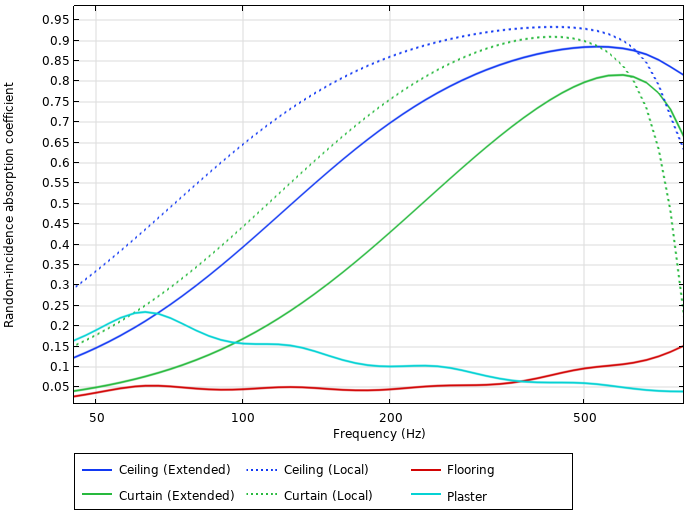Random incidence absorption coefficients for all materials used in the room model.

The ceiling and curtain show the different absorption coefficients for the different boundary models due to the high extended reactivity of these absorbers. The local reaction models show larger absorption coefficient values than the extended models over a wide frequency range, except above 630 Hz. You can see the angle-dependent absorption coefficients for the absorbing materials from the model file.

Normalizing and Filtering of the Impulse Response

Room acoustics metrics and auralization are used to evaluate room acoustics. Such evaluations are calculated from an impulse response, which is the response to a Dirac delta function with a flat spectrum over all frequencies. However, the direct implementation of the delta function leads to numerical instability. The approximated source models are used in actual simulations.

The Gaussian pulse is a typical source signal in wave-based, time-domain modeling, but its frequency spectrum is not flat, as will be shown later. Thus, to use dG-FEM results for room acoustics evaluation, the source spectrum needs to be normalized. Here, we introduce how to perform the normalization in the frequency domain.

First, we introduce the frequency characteristic of the Gaussian pulse. The Gaussian pulse was excited to sound fields with the following initial sound pressure distribution:

p=\exp(\frac{-r_{\rm s}^2}{d^2})

Here, p represents the sound pressure. r_{\rm s} is the distance from the source, and d is the parameter characterizing the source spectrum. Substituting this initial sound distribution function to the wave equation for a spherical wave yields the following relation in a free field (Ref. 2).

p({\bm r},t)=\frac{1}{2r_{\rm s}}(r_{\rm s}-ct)\exp(\frac{-(r_{\rm s}-ct)^2}{d^2})

Therein, t is the time variable, \bm r is the coordinate vector, and c is the sound speed. With the Green’s function for the three-dimensional free field, the volume acceleration of the point source \dot{Q} is expressed as follows (Ref. 3):

\dot{Q}(t)=\frac{2\pi}{\rho}(r_{\rm s}-ct)\exp(\frac{-(r_{\rm s}-ct)^2}{d^2})

Here, \rho is the density of the medium. By Fourier transformation, the spectrum of the source signal using the Gaussian pulse is expressed as follows:

\dot{Q}(f)=\frac{i\omega\pi^{3\over2}d^3}{\rho c^2}\exp(-(\frac{d^2\omega}{2c})^2)

Here, f is the frequency variable.

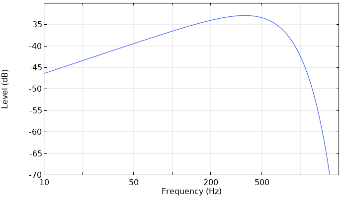The spectrum of the source signal used in the example model.

The source was designed so that the gain of -3 dB from the peak was obtained at the upper-limit frequency in the 500 Hz octave band.

Thus, we can obtain the normalized impulse response with a source strength of 1 m³/s² volume acceleration (around 0.14 mW source power in the air) by dividing the results by the analytic spectrum above. However, this normalization also amplifies the unwanted frequency components, such as a higher frequency component that is not resolved in the dG calculation. To remove such components, we also perform filtering. The following equation expresses the normalization procedure:

p_{\rm normalized}(t) = \mathcal{F}^{-1}[\frac{\mathcal{F}[p_{\rm dG}(t)]}{\dot{Q}(f)}HP(f)LP(f)]

Here, p_{\rm normalized} and p_{\rm dG} represent the normalized and dG-FEM-calculated sound pressure. \mathcal{F} is the Fourier transformation operator. HP and LP are the high-pass and the low-pass filters in the frequency domain, respectively.

Since the filtering process may result in a noncausal signal, zero padding is recommended before converting the dG results to the frequency domain via discrete Fourier transformation. The example model exported the pressure waveform calculated by the dG-FEM to a WAV file and imported it as an interpolation function. Then, zero padding was performed over the Grid 1D dataset as follows:

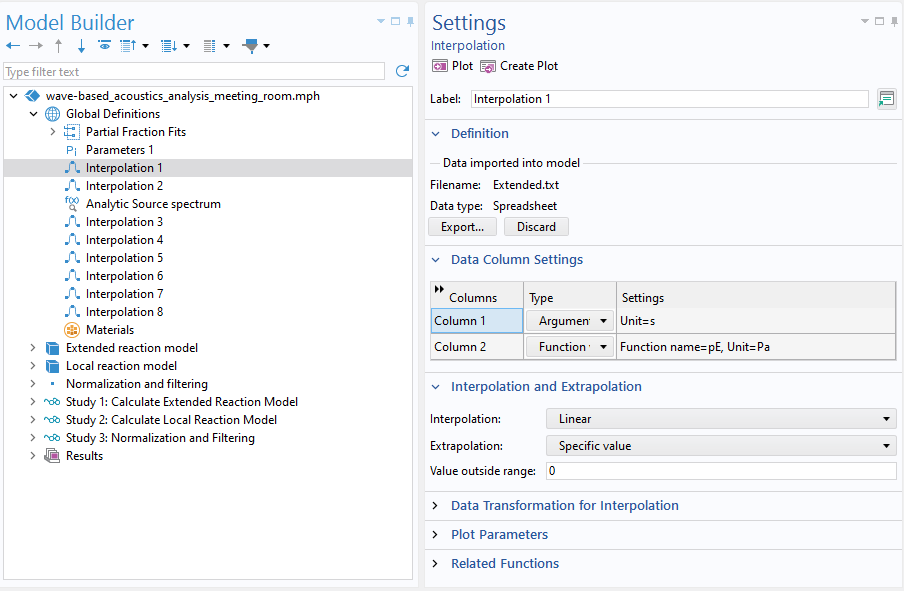Definition of an interpolation function using a WAV file exported from the calculation result. To perform the zero padding, the extrapolated value is set to 0.

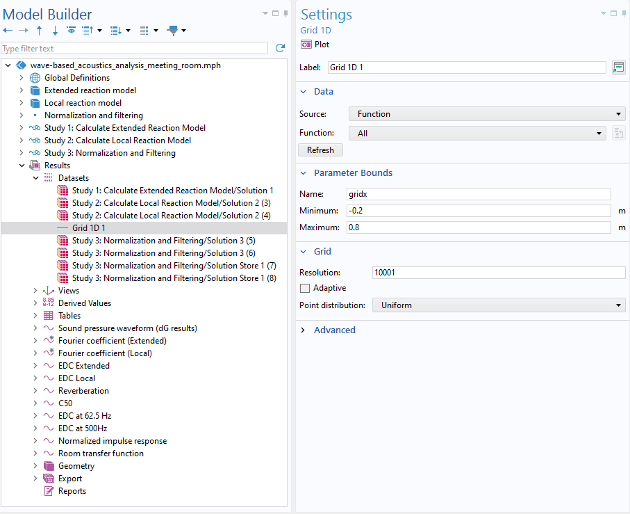Zero-padded Grid 1D for discrete Fourier transformation. The negative part of the interval is the zero-padded region. The resolution is set so that the sampling frequency corresponds to 10,000 Hz.

In the example model, the normalization and filtering were done with the following Global ODEs and DAEs interface.

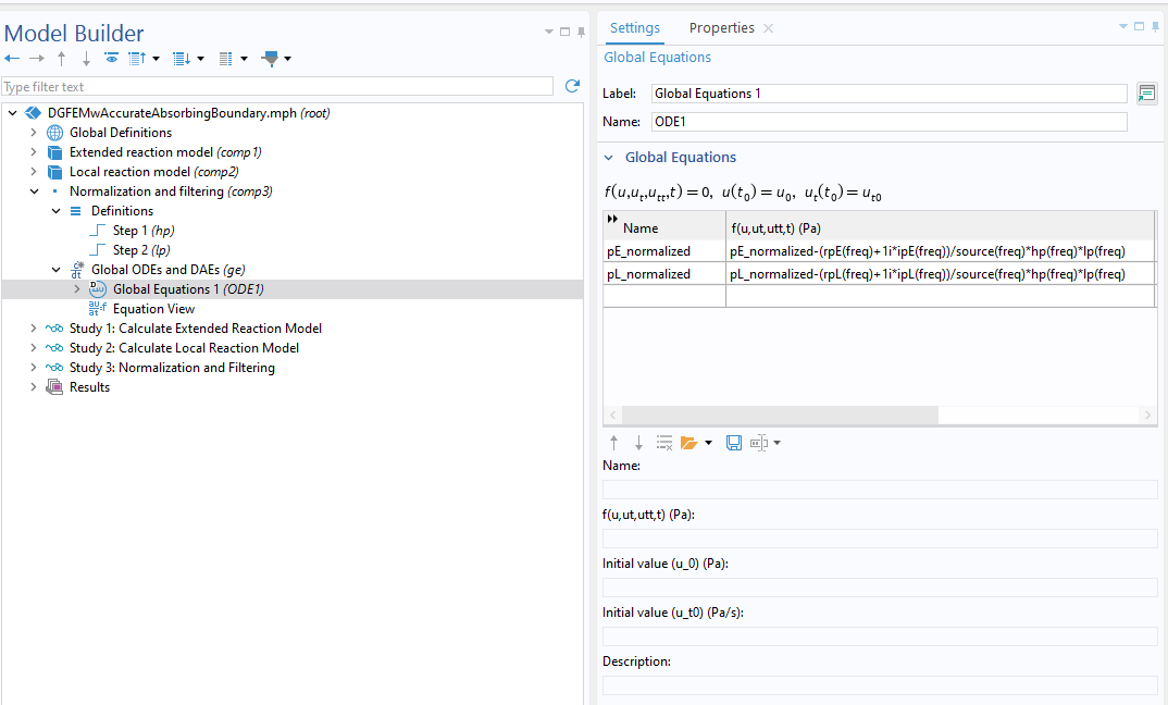Here, pE_normalized represents the normalized sound pressure, and rpE(freq) and ipE(freq) express, respectively, the real and imaginary part of the Fourier coefficient of the dG-FEM-calculated sound pressure for the extended reaction model. pL_normalized, rpL(freq), and ipL(freq) represent those same values, but for the local reaction model. source(freq) denotes the spectrum of the source signal defined with an analytic function. HP(freq) and LP(freq) are the high-pass and low-pass filters defined using step functions. You can see more detail of the setting from the example model. The frequency domain data of pE_normalized and pL_normalized are calculated using the Frequency Domain study step. Then, the normalized impulse responses are reconstructed via the Frequency to Time FFT study step.

Another benefit of the normalization is that the results can be combined with the ray acoustics model results to obtain the broadband impulse response using a hybrid approach. This is done by setting the ray release condition to be omnidirectional with the following total source power P_{\rm{src}}:

P_{\rm{src}}=\frac{Z_0\dot{Q}_{\rm U}^2}{8\pi c^2}

Here, \dot{Q}_{\rm U} is the unit volume acceleration of 1 m³/s².

Results

The normalized band-limited room impulse responses and their spectra (room transfer function) for two sound-absorbing boundary models are shown below.

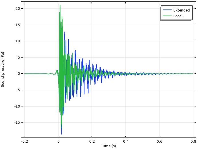Normalized room impulse responses for the extended and the local reaction models.

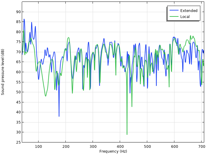Normalized room transfer function for the extended and the local reaction models.

The differences between the two models using different sound absorbing models are clear. The local reaction model overestimates the absorption by the sound-absorbing materials over a wide frequency range, which results in a faster decay of the impulse response. According to the comparison of the spectra, the local reaction model has more absorption below 160 Hz and around 500 Hz, while it underestimates the absorption above 600 Hz. These tendencies correspond to the differences in the random incidence absorption coefficients between two sound-absorbing boundary models.

The following comparisons of the room acoustics metrics also indicate the differences between the two models.

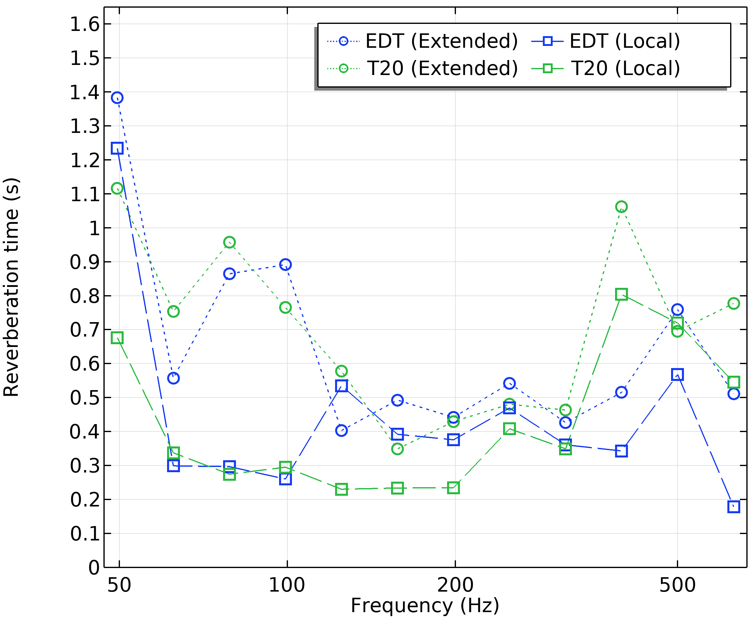A comparison of the reverberation parameters (EDT and T20) between the extended and local reaction models.

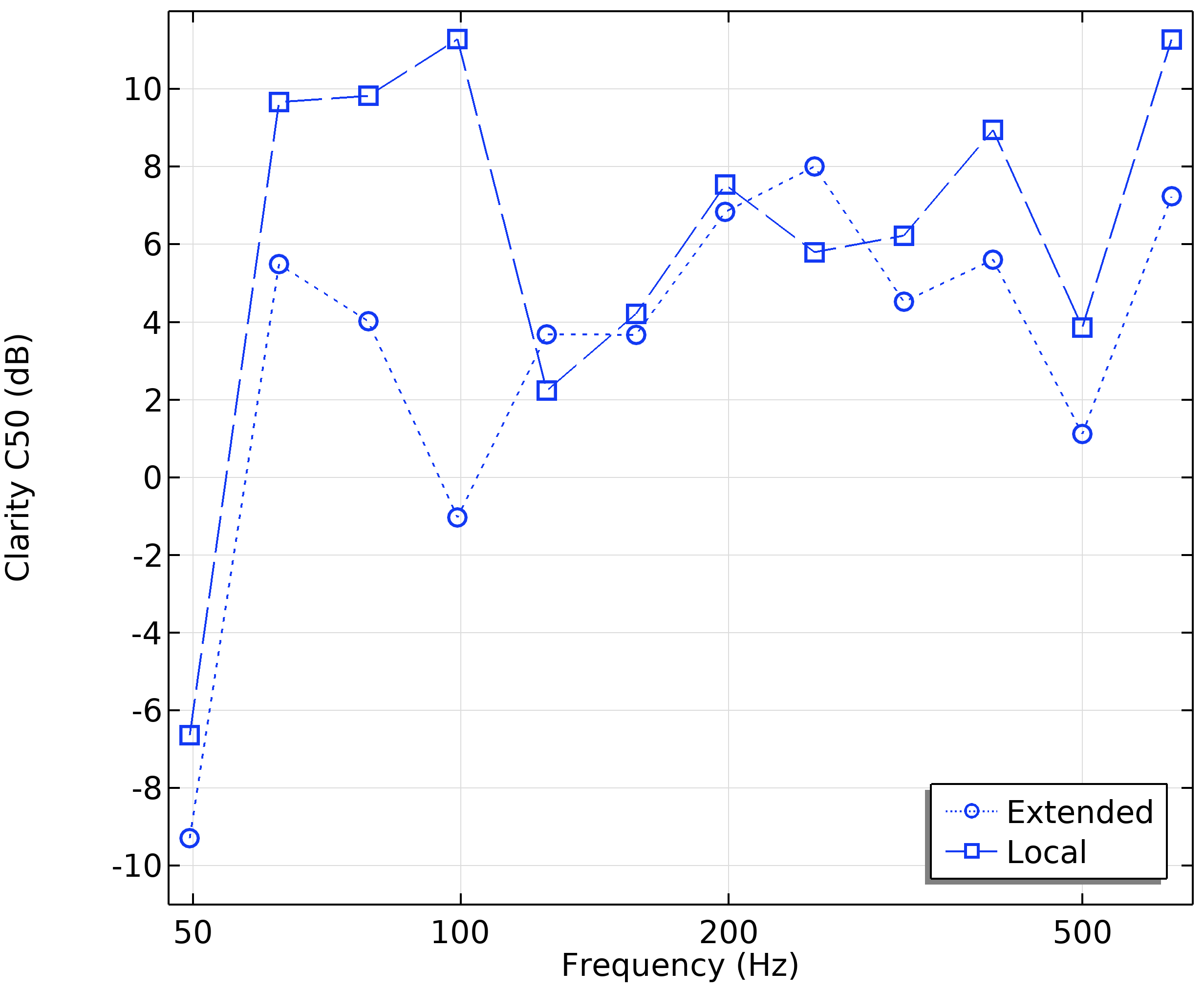A comparison of the clarity (C50) between the extended and local reaction models.

As for the reverberation parameters (EDT and T20), the differences between the two models are larger than the two times of just noticeable difference (JND) of 5% in a broadband. The clarity parameter (C50) also showed a larger difference than the JND (1.1 dB) at most frequencies, with the maximum difference reaching 11 dB. These results indicate that the difference between the local and the extended models is audible. You can hear the normalized and unnormalized room impulse responses for the different absorbing boundary models in the following:

Playback audio waveforms of the normalized impulse responses for the extended (left) and the local (right) reaction models.

Playback audio waveforms of the unnormalized impulse responses for the extended (left) and the local (right) reaction models.

You can feel the longer reverberation for the extended model. Also, the unnormalized results will be heard as emphasizing high-frequency sounds due to the frequency characteristic of the Gaussian pulse.

These results are at one receiver location, and it is important to set up more receiver locations for the practical evaluation of room acoustics. However, the clear differences at the possible receiver location are sufficient to demonstrate the effect of the type of the sound-absorbing boundaries on the meeting room.

The wave-based methods are considered to be inherently very accurate because they include all wave phenomena. However, the results of the example model showed that depending on the characteristics of the sound absorber, a simple use of the local reaction model may lead to erroneous results. In order to perform a more reliable simulation, we should carefully confirm the configuration and the absorption characteristics of the absorbers.

Conclusion

As a continuation of the previous blog post, this blog post examines the effects using different sound-absorbing boundary types on a small meeting room. Typical sound absorbing elements, like the suspended ceiling and the curtain, are highly extended reactive. As a result, applying the conventional local reaction model (the impedance boundary) to these absorbers produced a less accurate result. The demonstration revealed that the capability of the extended sound-absorbing boundary model is very crucial to perform a proper simulation. Of course, the impedance boundary is still convenient because of its lower computational cost than the extended model. For efficient modeling, the use of different absorbing models, depending on the design stage or the characteristics of absorbers, is very important. This blog post also introduced the procedure for obtaining a band-limited impulse response from the dG-FEM analysis with the Gaussian pulse excitation. Note that when exciting a sound field with the initial pressure distribution condition, the source location must be apart from any boundary surfaces reflecting sounds.

The Pressure Acoustics, Time Explicit interface in the Acoustics Module, an add-on to the COMSOL Multiphysics^® software, is well suited for wave-based room acoustics modeling because of its high-memory efficiency and accuracy, thanks to the ability to model both locally and extendedly reacting boundary models, including the frequency dependency. In addition, you can significantly reduce the computation time by using a GPU-accelerated formulation (currently available for only local reaction model). Even with an entry-level GPU (NVIDIA^® T400), the local reaction model (1,307,650 DOFs and 40,000 timesteps) can be solved in about an hour. If you have a higher-grade graphics card, the reduction of computation time is expected to be much greater. You can find more details about the performance gain by GPU in the following document: Acoustics of an Open-Plan Office Space.

Let’s model room acoustics with the exceptionally accurate and efficient simulation capabilities available in COMSOL Multiphysics^®!

Next Steps

Interested in trying out the model for yourself? Download the related MPH file below:

Try The Model

Reference

H. Wang and M. Hornikx, “Extended reacting boundary modeling of porous materials with thin coverings for time-domain room acoustic simulations,” J. Sound Vib., vol. 548, 117550, 2023; https://doi.org/10.1016/j.jsv.2022.117550.
S. Sakamoto, “Phase-error analysis of high-order finite difference time domain scheme and its influence on calculation results of impulse response in closed sound field,” Acoust. Sci. Technol., vol. 28, 295-309, 2007; https://doi.org/10.1250/ast.28.295.
T. Okuzono, T. Otsuru, R. Tomiku, and N. Okamoto, “Application of modiﬁed integration rule to time-domain ﬁnite-element acoustic simulation of rooms,” J. Acoust. Soc. Am., 1vol. 32, 804–813, 2012; https://doi.org/10.1121/1.4730920.