

Various machinery, such as engines, pumps, and turbines, employ components that transmit the load between the solid parts that are in relative motion. Common examples are piston rings, cams, gear teeth, and (of course) bearings. Often, these components are lubricated by maintaining an oil film between the two solid parts to minimize the friction and wear. In this blog post, we look at methods for modeling the fluid friction in lubricated joints.
Modes of Lubrication
Depending on the loads between the two contact surfaces and their geometry, the following different regimes of lubrication can be observed:
- Fluid-film lubrication
- The load is fully supported by the fluid film such that the contacting surfaces are fairly separated by the fluid film
- Elastohydrodynamic lubrication
- Observed between nonconforming surfaces or high load conditions, where the bodies suffer significant elastic strain at contact
- Fluid film is still maintained between the deforming surfaces due to the pumping action of the relative motion between the surfaces
- Boundary lubrication
- The bodies come into closer contact at their asperities, and hydrodynamic effects are negligible
- Mixed lubrication
- A regime between the full-film elastohydrodynamic lubrication and boundary lubrication, where the lubricant film alone is not enough to separate the bodies completely
- Hydrodynamic effects are considerable
In this blog post, we will focus on the full-film lubrication regimes, because joints form conforming surfaces and the pressure is not high enough to cause significant deformation.
Calculating the Viscous Drag Force Between Plates Separated by a Lubricant
Consider two flat plates separated by a lubricant, as shown in the figure below. The bottom plate is kept fixed and the top surface moves by a horizontal velocity, U.
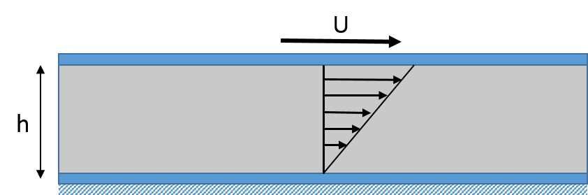
Shear flow between two flat plates.
For a Couette flow without the pressure gradient, the velocity profile of the lubricant in the thickness direction z can be written as:
Therefore, the viscous shear stress in the lubricant is:
which is independent of the thickness coordinate.
Thus, the viscous shear drag on the top plate is given by:
where A is the area of the plate.
In the case of joints, the lubricant flow also has a pressure gradient due to the varying thickness of the film. In such a case, the velocity profile changes to:
where x is the coordinate along the direction of the flow.
In this case, the viscous shear stress at the top plate is given by:
and the viscous shear drag on the same is:
Determining the Viscous Force in Lubricated Joints
To understand the viscous force in joints, let us take the example of a hinge joint. The hinge joint is a joint that allows the relative rotation about the joint axis between the two components forming the joint. In general, as opposed to the above example, both of the components forming the hinge joint can be in motion; for instance, a joint between the connecting rod and crank pin of a reciprocating engine. A general scenario is shown in the figure below, where the components are rotating about their center at speeds Ω1 and Ω2, respectively. If the inner radius of component 1 is R1 and the outer radius of component 2 is R2, then the surfaces are moving at speeds Ω1R1 and Ω2R2, respectively.
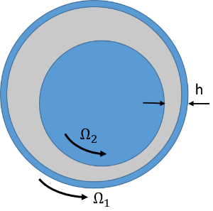
Lubricated hinge joint.
At any location locally, the flow is similar to the one described for the flat plate. Therefore, the velocity profile at any circumferential location of the film in the tangential direction is given by:
where the subscript t represents the tangential component and z is measured from component 2.
The viscous shear stress in the lubricant then is:
Assuming that Ω1R1 > Ω2R2, the shear stress at surface 1 is:
and at surface 2 is:
Then, the total drag force on both surfaces is obtained by integrating the shear stress on the surface as:
F_{f2} &= \int_0^L\int_0^{2\pi}\tau_2dxd(R_2\phi)=\mu R_2(\Omega_1R_1-\Omega_2R_2)\int_0^L\int_0^{2\pi}\frac{dx}{h}d\phi-\int_0^L\int_0^{2\pi}\frac{h}{2}\frac{\partial p}{\partial \phi}dx d\phi
\end{aligned}
Modeling Lubricated Joints in COMSOL Multiphysics®
Joints are available in the Multibody Dynamics Module, an add-on to the Structural Mechanics Module and the COMSOL Multiphysics® software. These joints can either be rigid or flexible joints. Rigid joints, as the name suggests, do not allow any relative motion between the components other than the joint degrees of freedom (DOFs). In flexible joints, you can specify the stiffness between the components for the relative motions other than the joint DOFs. This stiffness can be due to the flexibility of the components themselves, the presence of a fluid film between the area forming the joint, or a combination of both. It is the effect of the fluid film that we wish to address here.
A lubricant in the joint supports the joint forces through the film pressure, thus avoiding the structure-to-structure contact and reducing the friction between the joint components. Although not as large as contact friction force, shearing of the lubricant due to the relative motion in the joints offers a resistance to the relative motion on both of the components forming the joint. This resistance is what we call fluid friction in joints. Therefore, a fluid film in the joint applies two types of forces on the joint components:
- Force to support the load on the joint
- Viscous shear force to resist the relative motion of the components
Therefore, the simplest way of accounting for the support forces of the fluid film is by using dynamic characteristics (stiffness and damping coefficient) of the fluid film as the joint stiffness and viscous damping in an elastic joint. Often, these characteristics are known through some experiments. For simple cases, analytical expressions as a function of the eccentricity are also available for the dynamic characteristics of the bearing. COMSOL Multiphysics also provides a way to compute the dynamic characteristics of the lubricant film in the joint via the Hydrodynamic Bearing interface. This interface is available in the Rotordynamics Module (also an add-on to COMSOL Multiphysics and the Structural Mechanics Module), which is used for simulating the flow in fluid-film bearings. In addition, to account for the viscous resistance, a joint force (or moment) should be applied to the relative motion in the joint. The method to calculate the viscous resistance is explained in the previous section.
Calculating the dynamic coefficients and viscous resistance for each joint and using it in a multibody simulation can be a rather tedious process. There is an easier way of modeling the joint lubrication in the COMSOL® software. A multiphysics coupling feature called Solid Bearing Coupling is provided to combine the hydrodynamic bearing simulations directly with the multibody and structural mechanics ones. The coupling feature transfers the motion of the structure to the Hydrodynamic Bearing interface to compute the change in the film thickness, which affects the pressure distribution in the film. The pressure and shear forces in the film are then transferred back to the structure as an external force, making it a bidirectional coupling.
An Example of Fluid Friction in Joints
To understand the modeling process explained above, let’s take a look at an example. Consider a piston and cylinder of a reciprocating engine. The walls of the piston and cylinder are separated by a thin lubricant film, as shown in the figure below.
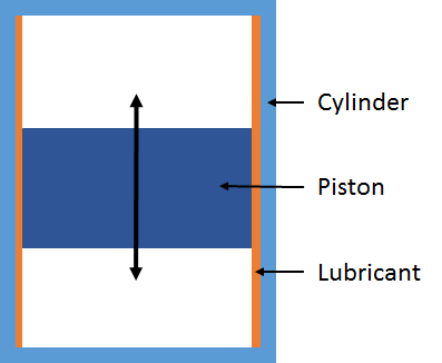
Lubrication of a piston reciprocating in a cylinder.
The piston is connected to the connecting rod, which is connected to the crankpin on the other end. The schematic of the whole system is shown in figure below:
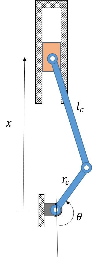
Schematic of a slider crank system.
The radius of the crank is rc, and it rotates at an angular speed Ω. The length of the connecting rod is lc. From the geometric considerations, the vertical position of the piston from the crank center is given by
where θ = Ωt.
In the above expression, θ is referred from the crank position when the piston is at bottom dead center (BDC).
The initial position of the piston (at BDC) from the crank center is
Therefore, the vertical displacement of the piston is given by:
Note that at t = 0, the displacement and velocity of the piston are 0.
Let us further assume that a vertical force due to gas pressure is acting on the piston, given by
Thus, the force is zero when the piston is at bottom dead center and is maximum when it is at the top dead center. In a real scenario, this force will have a more complex dependence on θ. The connecting rod supports this load through its reaction on the piston. Interestingly, this reaction, Fc, is always along the length of the connecting rod, as shown in the figure below.
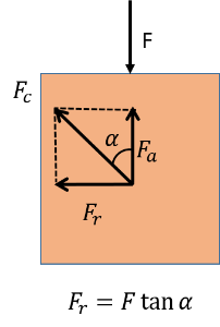
Free body diagram of a piston.
Thus, the vertical component of the reaction, Fa, supports the gas pressure on the piston. However, there is an additional horizontal component, Fr, acting on the piston. It pushes the piston to the cylinder walls. This force, whose magnitude is given by
also needs to be applied on the piston as it moves in the cylinder.
To simulate such a problem, we start by creating a geometry of the piston. We can use the Linear Elastic Material model in the Solid Mechanics interface to model the flexibility of the piston. The motion of the piston is prescribed using the Rigid Connector feature, also available in the Solid Mechanics interface. Motion of the piston in the vertical direction (z direction) is prescribed as obtained from the geometric considerations above. Also, the piston cannot rotate about its axis (z-axis). Lateral translation and tilting of the piston are set free, which will be obtained from the force balance on the piston. These conditions can be specified using a setting, shown in the image below, in the Rigid Connector feature.
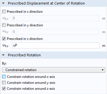
Screenshot showing the prescribed motion and displacement of the piston.
The horizontal load on the piston coming from the connecting rod is modeled using the Applied Force subfeature on the Rigid Connector feature.
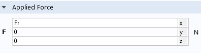
Screenshot showing the Applied Force feature and its settings.
Computation of the fluid friction on the piston requires the evaluation of resistive force to the motion of the piston from the lubricant film. Although we could model the cylinder and piston together (with the lubricant between them), it is not necessary to model the cylinder because it remains stationary. The stationary state of the cylinder can be directly specified in the Hydrodynamic Bearing interface.
Due to lateral motion of the piston, the gap between the piston and cylinder changes, which will effectively change the lubricant’s thickness. Thus, the pressure distribution in the lubricant film also depends on the relative motion of the contacting boundaries. Under high loads, deformation in the piston can also change the film thickness. If the ratio of the pressure in the film to the effective stiffness of the contacting boundaries is small, the deformation during the contact can be neglected. Otherwise, deformation of the contacting boundaries needs to be considered because it plays a significant role in determining the effective friction between the contacting boundaries. Simulation of this class of problem is classified as elastohydrodynamic (EHD) simulation. In this case, since the pressure levels are expected to be low, film thickness will largely be affected by the lateral motion of the piston rather than its deformation.
To model the lubricant film, we make a thin-film approximation of the Navier-Stokes and continuity equations to get the Reynolds equation, which is solved on the surface instead of the fluid domain. The Hydrodynamic Bearing interface solves the Reynolds equation and can be used for getting the pressure distribution in the film on the piston surface. Parameters required for the modeling of the lubricant film are the initial film thickness, viscosity and density of the lubricant, and motion of the contacting boundaries. All of this information is specified in the Hydrodynamic Journal Bearing feature of the Hydrodynamic Bearing interface.
Note that the Hydrodynamic Journal Bearing feature, in general, can model a journal bearing where the journal undergoes an axial rotation in addition to its translational motion. This feature can also be used in cases where there is no axial rotation of the journal, like the piston in the present model. The motion of the contacting boundaries can be easily passed to the Hydrodynamic Journal Bearing feature using the built-in Solid-Bearing Coupling multiphysics feature. As mentioned in the previous section, this feature automatically applies the forces due to the pressure and shear of the lubricant in the film on the structural boundary.
Visualizing the Simulation Results
The animations below show the pressure distribution in the film and the stress in the piston as the part performs the reciprocating motion. To highlight the lateral motion of the piston, the reciprocating motion of the piston is suppressed.
The von Mises stress in the piston (left) and the pressure in the film (right).
You can see the flipping of the stress after the half cycle of the piston. Note that during the upward stroke, as the connecting rod pushes the piston on the right wall, the pressure increases on the right side of the piston and decreases on the left side. During the downward stroke, the direction is reversed.
The time variation of force on the piston in the vertical direction due to the shearing of the lubricant film is given in the figure below.
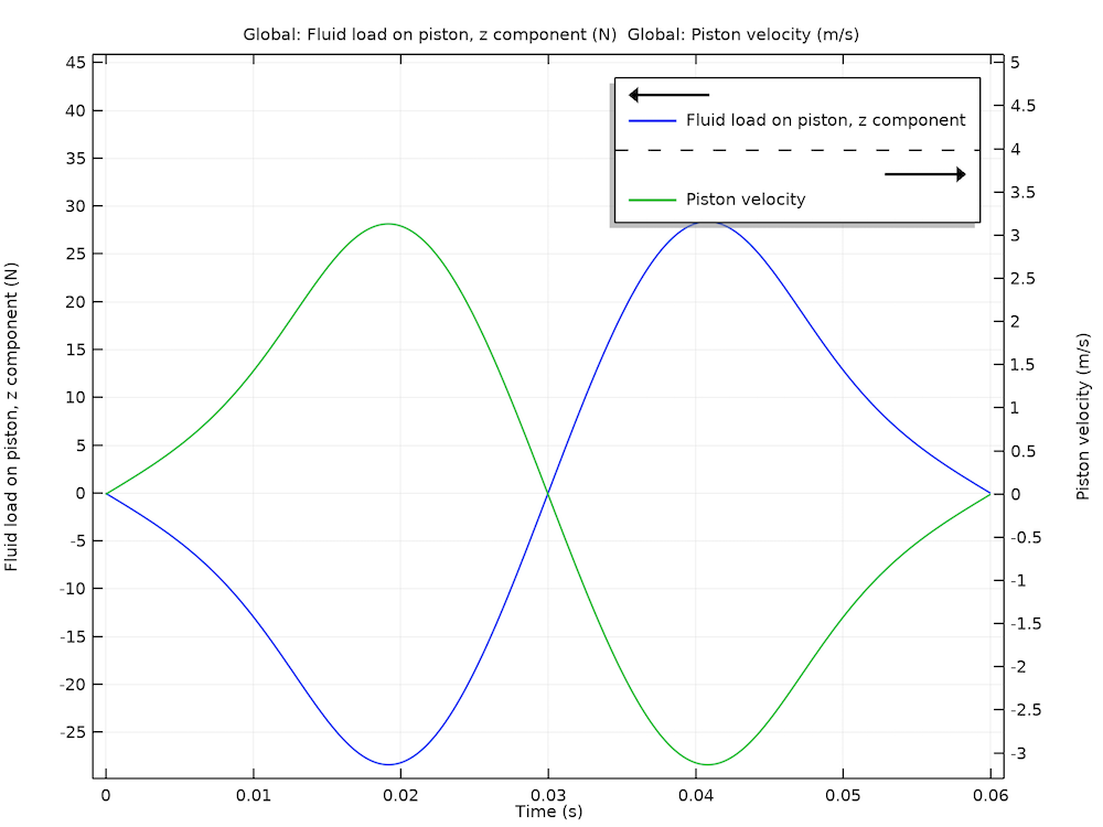
Piston velocity and viscous force.
Note that the viscous force on the piston is always opposite of its velocity. The viscous force coefficient (damping coefficient) is given by the ratio of the viscous force to the piston velocity. In the present case, it is approximately 8 N*s/m.
Reciprocating Engine Example
The Reciprocating Engine with Hydrodynamic Bearings model, available in the Application Library with the Rotordynamics Module, demonstrates the steps of combining the structural or multibody simulation with the hydrodynamic bearings. In this example, a single-cylinder reciprocating engine supported through hydrodynamic journal bearings on the foundation is considered. The dynamics of the various engine components are analyzed when gas pressure is applied on the piston. During the engine’s operation, the load on the piston is transferred to the foundation through the connecting rod, crank, and bearings.
The pressure in the bearings and the stress in the foundations are analyzed to understand the bearing performance and the stress variation on the foundation during one operating cycle. The stress in the crankshaft is also analyzed. The animation below shows the stress variation in the crankshaft and foundation as well as the resulting bearing pressure distribution during its operation. Bearing pressure is highest during the downward stroke of the piston under the gas pressure.
Reciprocating engine: stresses in the crankshaft and foundation as well as pressure in the bearing.
The viscous torque on the bearing is plotted for various cycles of operation. As the piston reaches the top dead center, the cylinder pressure is highest. At this instant, the pressure in the bearing is also very high and the eccentricity of the journal is at maximum. This creates high friction on the journal, which appears as sharp negative peaks in the viscous torque plot. Note that the viscous torque is approximately 10% of the loading torque (approximately 16 Nm), which is quite significant and cannot be ignored when computing the losses in the engine.


The viscous torque in the bearing (left) as well as the driving and loading torques on the crankshaft (right).
Next Steps
Learn more about the specialized features for modeling the characteristics of thin-film lubricant flow available in the Rotordynamics Module by clicking the button below.
Note that this product (as well as the Multibody Dynamics Module) is an add-on to the Structural Mechanics Module and COMSOL Multiphysics.
Further Reading
- Read more about modeling bearings on the COMSOL Blog:


Comments (0)