Is the boundary element method (BEM) a viable alternative to FEM for magnetostatics modeling? In a three-part series of tutorials, we perform electromagnetic force calculations using the Maxwell stress tensor to demonstrate the capabilities of BEM. The results are validated against analytical models and compared with results from FEM to show the value and utility of boundary elements for this purpose. Read on for a preview of what you’ll learn in the tutorial series.
Comparing Boundary Elements and Finite Elements
BEM is a numerical modeling tool that can be used instead of (or combined with) FEM for the analysis of electrostatics, magnetostatics, acoustics, corrosion, and more. Unlike FEM, BEM requires a surface mesh only, so the generation of a volumetric mesh throughout the computational domain is unnecessary.
BEM can be computationally efficient and easy to implement — when applied under the right circumstances. The method connects every degree of freedom with every other degree of freedom and works well for infinite domains, isotropic materials, and wires. However, BEM is not applicable for models with nonlinear or general inhomogeneous materials.
Take electrostatics as an example. In this area, a variety of modeling tasks can be streamlined by using BEM, including:
- Modeling wires and isotropic materials
- Setting up infinite domains
- Postprocessing at arbitrary distances
In some cases, you can model some regions with BEM, model some domains with FEM, and then combine the two methods to experience the benefits of each.
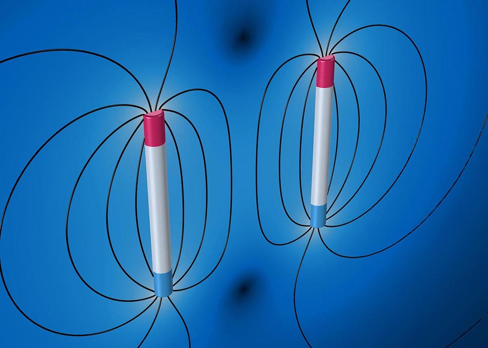
A model of two parallel magnetic rods from the Electromagnetic Force Verification tutorial series.
Now that you have a basic rundown of BEM, you might be wondering what can you do with it. For one, this method is advantageous when accurate flux computation is important. In this series of tutorials, we investigate BEM as an alternative to FEM within the context of magnetostatics modeling — particularly for computing electromagnetic forces using the Maxwell stress tensor.
Let’s see how well BEM performs in comparison to FEM and then validate the approach with an analytical model.
Performing and Validating Electromagnetic Force Calculations
For this tutorial series, the following products have been used: the COMSOL Multiphysics® platform and the add-on AC/DC Module. Some of the techniques for verifying electromagnetic analyses in the tutorials include:
- Using fillets, advanced meshing, and exterior force-probe surfaces to increase accuracy
- Comparing BEM and FEM for several mesh sizes
- Investigating mesh convergence via parametric sweeps
Part 1 of the series introduces you to the model geometries that will be used in parts 2 and 3 and gives detailed instructions on how to build them step by step.
Note: More experienced software users can skip the introduction in Part 1 and move on to Part 2. If you’re new to COMSOL Multiphysics, these instructions will help you get started with the basics of setting up a model geometry.
The model geometry in Part 2 is made up of a single rod in a semisphere with a second rod accounted for via symmetry. For the torque analysis in Part 3, a single rod is placed in a spherical domain and encapsulated by a cubic surface, which applies an external field to the rod.
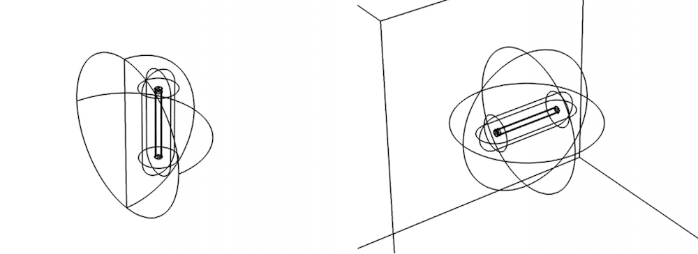
The model geometry for the electromagnetic force (left) and electromagnetic torque (right) models.
Calculating Magnetic Force with a Hybrid BEM–FEM Approach
There are many different ways to determine the electromagnetic force on a rigid body. When computing the forces using the Maxwell surface stress tensor, it is important to have accurate flux integrals for the magnetic field (H) and magnetic flux density (B).
BEM is quite strong in this area, offering a potential advantage when calculating force. Unlike with FEM, when using BEM, the flux normal to the boundary is entered directly as a degree of freedom, which allows for accurate flux computation without requiring reaction force integrals or weak constraints. By solving the models discussed here using BEM and comparing the results to FEM and analytical models, we can validate the use of BEM for electromagnetic force computations.
When it comes to magnetostatics, two theoretical constructs are prevalent:
- Magnetic poles
- Atomic currents
We base the analytical model used here on magnetic poles, as it considers the static magnetic charge and is mathematically equivalent to electrostatics.


2D geometry of the electromagnetic force verification model (left) and the analytical model for verification (right).
The verification model includes two magnetized rods that are both 1 meter long and 1 meter apart. The remanent flux density inside the rods is specifically chosen, such that the analytical model predicts a repelling force between the rods of exactly 1 Newton-meter. These conditions are important because we can use them to compare the numerical results and determine their level of accuracy.
Comparing 2 Methods for Electromagnetic Force Calculations
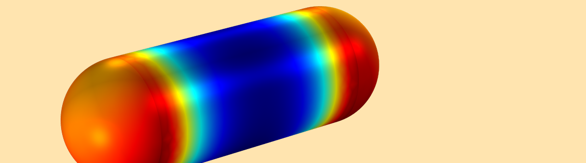
Looking at the results, we see that the BEM approach can produce smooth fields, even for models with a relatively coarse mesh.


The Maxwell surface stress tensor, used to compute the electromagnetic force, at the rod surface (left) and probe surface (right).
When comparing the BEM and FEM results to the analytical model for different mesh sizes (see graph below), we see that on one hand, the boundary element method produces accurate results for coarse meshes. The finite element method, on the other hand, requires much finer meshes on the poles to reach the same level of accuracy.
In addition, note that the results for the force probe are more accurate. The stress tensor behaves much more nicely at a certain distance from the magnet, which is why the force probe model compares nicely with the analytical model.
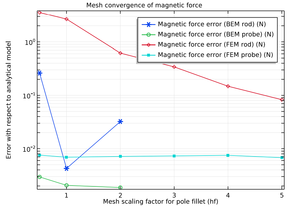
Relative margin of error of the force calculations for the rod surface using BEM (dark blue), probe surface using BEM (green), rod surface using BEM–FEM (red), and probe surface using BEM–FEM (light blue).
The simulation results also show that the stresses are strongly concentrated on the fillets of the magnet, which explains why calculating forces on rigid bodies with sharp edges is, in general, inaccurate. In fact, computing forces on magnets with sharp corners could lead to results that are off by as much as 2000%. The BEM approach can produce smooth fields for your results, even for models with a relatively coarse mesh.
Analyzing Magnetic Torque with the Boundary Element Method
Part 3 continues the analysis of the Magnetic Force BEM-FEM verification model with a different geometry. A single magnetized rod that is one meter long is placed in a perpendicular external field Be (below, to the right). The strength of the external field is chosen such that the analytical model predicts a torque on the rod of one Newton-meter exactly. This way, we can use the analytical model to validate the numerical results for the torque on the rod.


Schematics of the model geometry (left) and analytical model (right) for the torque analysis.
For the BEM approach, the results are similar to those for the electromagnetic force tutorial. There are smooth fields with coarse meshes, the stresses are concentrated at the fillets, and there is decent accuracy when compared to the analytical model.


The Maxwell surface stress tensor, used to compute the electromagnetic torque, at the rod surface (left) and probe surface (right).
The results for the combined BEM–FEM approach have a larger margin of error, much like in Part 2. For both the BEM and combined approaches, the probe surface results are also more accurate than the rod surface results.
As demonstrated through these two models, BEM can be advantageous for magnetostatics modeling when used properly and applied under the right circumstances.
Next Steps
Follow along with the Electromagnetic Force Verification Series for a comprehensive look at performing and validating electromagnetic force calculations. You can access the PDF instructions and MPH file downloads by clicking the button below, which will take you to the Application Gallery.
Further Reading
Find more information about electromagnetics modeling in these related blog posts:


Comments (0)