
No matter how much you refine the mesh at that corner in your geometry, the electromagnetic field that you are computing never seems to settle on a converged value. Is this a problem? If so, what can you do about it? Read on to find out.
Singular Electromagnetic Fields at Sharp Edges
Let’s look at a model of a bent copper wire. You have applied a voltage of 5 mV between its ends, and the model computes the resulting total current running through it. With the default Normal mesh, you get a current of 490 A. You decide to try a few other mesh settings in order to determine the accuracy of this current. The results vary only by a few mA and there is markedly less variation between the finer mesh cases. You judge that the result is mesh convergent and sufficiently accurate for your needs.
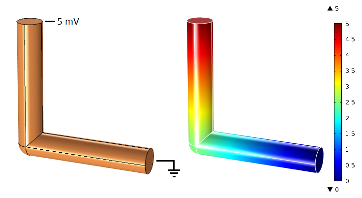
Wire model setup (left) and computed electric potential distribution in mV (right).
Next, you evaluate the maximum current density in the wire. It is important that this value isn’t too high. If it is, the resulting heat production risks wearing out the protective jacket and can even be a potential fire hazard.
The normal mesh gives you a maximum current density of 6.2 A/mm2. It is clear that this value appears at the inside corner of the bend, so this time you take care to refine the mesh within that area. The graph below shows the (quite alarming) results: Even if you refine the mesh by a factor of 100, the maximum current density is still growing and there is no indication that it will ever stop.
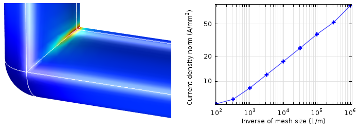
Singular current density at the inside corner (left) and calculated maximum current density vs. local mesh density (right).
What you have run into is a geometrically singular result. The current density is proportional to the electric field, which in turn is (the negative of) the gradient of the electric potential. While the electric potential itself remains smooth and well-defined at a sharp corner, its gradient is in theory infinite. Numerically, it will tend toward infinity as you refine the mesh. In reality, there are of course no perfectly sharp edges. However, the sharper the edge, the greater the local current density.
Creating Fillets in COMSOL Multiphysics®
If you give the edge a finite radius of curvature, you can limit the current density in the model to simulate reality far better.
Here’s how you do it:
- Create a union of the objects that intersect the edge, making sure to clear the Keep interior boundaries check box. This makes the direction of the fillet unambiguous.
- Add a Fillet node. Select the edges you want to include and supply a suitable radius.
- Click Build All Objects to see the result.
With the fillet in place, the model now returns a smooth current distribution, with a convergent maximum value of 5.1 A/mm2.
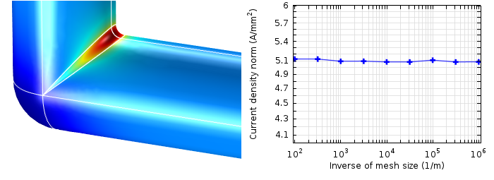
Smooth current density distribution (left) and calculated maximum current density vs. mesh density on the fillet (right).
To Fillet or Not to Fillet?
If you are only interested in the total current, voltage distribution, or the current density some distance away from the singularity, then you can get good results even without the fillets. This, importantly, also goes for lumped parameters such as resistances and impedances. In an electromagnetic heating model, even a small thermal conductivity is sufficient to give a smooth temperature distribution and a convergent maximum temperature despite a locally singular current density.
Still, if you want to ensure that you get your local fields and currents right, keeping it smooth is a good idea. In general, edges and corners in 3D, as well as corners in 2D, may give you singular electric or magnetic fields. This holds true if they both demark the outer limits of your model or if they separate materials with different properties. If the fields are singular, so are most of the variables that depend explicitly and locally on them.
The next image shows the Maxwell stress tensor on the surface of an iron bar next to a horseshoe magnet. As the stress tensor is proportional to the magnetic field squared, it becomes singular if the bar has sharp corners and edges.
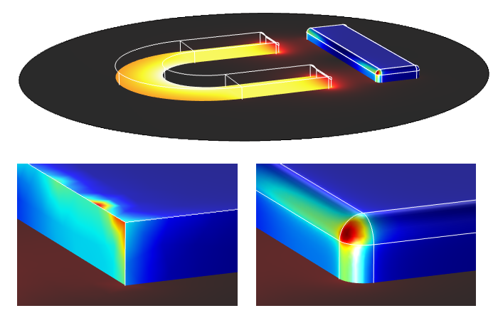
Magnetic flux density around a horseshoe magnet and Maxwell stress tensor distribution on a nearby iron rod. The close-ups show the local flux density on the iron bar without (left) and with (right) fillets.
Outside of electromagnetics, many other solution-variable gradients (heat fluxes, stresses, strains, etc.) exhibit similar singularities and will become smooth if you fillet your edges and corners. You can read more in this previous blog post on singularities.
Resist Temptation…
Last but not least: Don’t cut corners! It may be tempting to keep the total mesh count down by using the simpler Chamfer operation instead of applying fillets. This, however, gives you a straight section instead of the smooth bend and literally replaces each singularity you remove with at least two additional ones.
Fillets (and chamfers) in 2D are included in the COMSOL Multiphysics® software as of version 5.0. In 3D, you need the Design Module.


Comments (2)
Mohammad Wahiduzzaman Khan
October 21, 2018This helped a lot, thank you! But sometimes, I find it hard to do optimized meshing (too long to converge) with fillet in the geometry. Is there any suggestion on that?
Brianne Costa
October 29, 2018 COMSOL EmployeeHello Mohammad,
Thanks for your comment.
For questions related to your modeling, please contact our Support team.
Online Support Center: https://www.comsol.com/support
Email: support@comsol.com