
Electron transport in low-temperature plasmas depends strongly on the electron energy distribution function (EEDF), which is often approximated as Maxwellian but is frequently nonequilibrium in reality. Incorporating nonequilibrium EEDF behavior into spatially dependent models often requires precomputed multidimensional lookup tables or the self-consistent solution of the Boltzmann equation during the simulation. This blog post presents a more efficient alternative: a deep neural network surrogate model trained on Boltzmann equation solutions. This enables accurate integration of kinetic effects into fluid plasma simulations while significantly reducing computational cost.
Methodologies for Embedding Kinetic Data in Space-Dependent Fluid Dynamics Models
In cold plasmas, electron transport properties and source terms are highly sensitive to the electron energy distribution function (EEDF). For simplicity, a Maxwellian or other analytical EEDF is often assumed. However, in many practical situations, electrons are far from equilibrium, and a more accurate representation of the EEDF is required to obtain realistic simulation results.
A common and effective method for computing the EEDF in low-temperature plasmas is to solve the Boltzmann equation using the two-term approximation. These computed EEDFs can then be imported into spatially dependent models, as described in a previous blog post: The Boltzmann Equation, Two-Term Approximation Interface. This approach is both efficient and convenient, but it has a major limitation: The resulting EEDFs are only functions of the electron mean energy. As a result, variations due to changes in gas composition (mole fractions) and ionization degree cannot be captured.
At the other end of the complexity spectrum, the Plasma Module, an add-on to COMSOL Multiphysics®, offers the ability to solve the Boltzmann equation (in the two-term approximation) fully coupled with a spatially and temporally resolved plasma fluid model. This method, as demonstrated in the GEC ICP Reactor model, automatically accounts for variations in gas composition (including excited states), ionization degree, and other factors. However, this fully coupled approach comes with a significantly higher computational cost.
A third approach is to develop a deep neural network surrogate model trained on data generated from the Boltzmann equation solved using the two-term approximation. Once trained, the DNN can be integrated directly into spatially dependent plasma simulations to reproduce kinetic effects with near-Boltzmann accuracy. By combining the precision of kinetic modeling with the computational efficiency of fluid models, this hybrid method offers an effective balance between accuracy and performance.
Creating the Data for the Surrogate Model
The first step is to have a space-dependent plasma model that solves well using an analytic EEDF. In this example, we use a model of an inductively coupled plasma reactor in argon. Within the same MPH file, add a 0D component along with the Boltzmann Equation, Two-Term Approximation interface. This interface generates the data necessary to build the surrogate model.
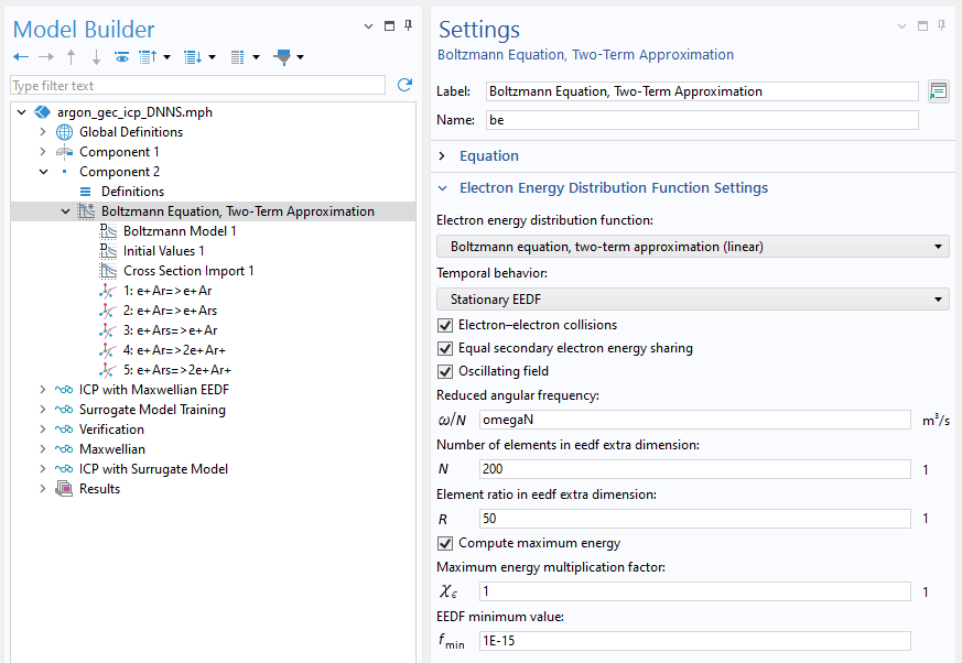 Settings of the Boltzmann Equation, Two-Term Approximation interface.
It is important that the electron impact reactions defined in the Boltzmann Equation, Two-Term Approximation interface and the Plasma interface are consistent but not necessarily identical. For example, solving the approximated Boltzmann equation can have a detailed set of electron impact reactions, while the Plasma interface might include a simplified single reaction representing total ionization. In this example, we use a one-to-one matching between reactions.
Next, add a new study to compute the data required for training the surrogate model. Within this study, include a Surrogate Model Training node. This node allows you to select training settings and define output quantities (or quantities of interest). The actual training is done in the Deep Neural Network node, which is automatically generated after running the study.
For the Surrogate Model Training node, it is important to:
- Set the surrogate model type to Deep Neural Network
- Set the layers for the deep neural network and activation function
- Define the quantities of interest and use Configure study-dependent input for all
- Set the input parameters and sampling strategy
The quantities of interest correspond to the surrogate model outputs used later in the spatially dependent plasma model. For this example, these include functions for all electron impact rate constants, reduced electron mobility, effective reduced electron collision frequency, and the field coefficient. Note that the reduced electron mobility refers to the DC mobility used for in-plane electron transport, while the effective collision frequency and field factor contribute to computing plasma conductivity (as detailed in Ref. 1).
The choice of input parameters must be tailored to each specific case. For this example, in addition to the always required electron mean energy parameterization, we also sample the ionization degree (Beta), defined as the ratio of electron density to gas density, and the mole fraction of the argon excited state (xArs). To effectively capture how these inputs influence the outputs, only a few sample points per decade are needed, which we achieve through uniform sampling in the logarithmic domain.
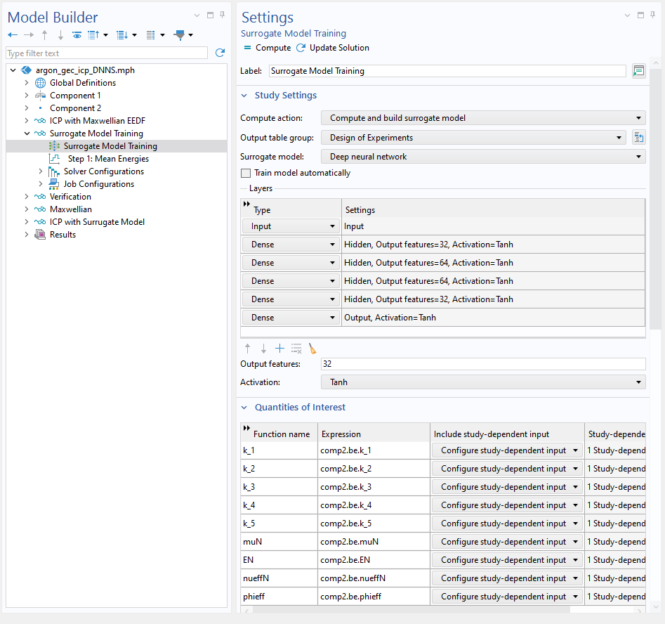 Settings of the Surrogate Model Training node showing the layers of the DNN and the quantities of interest.
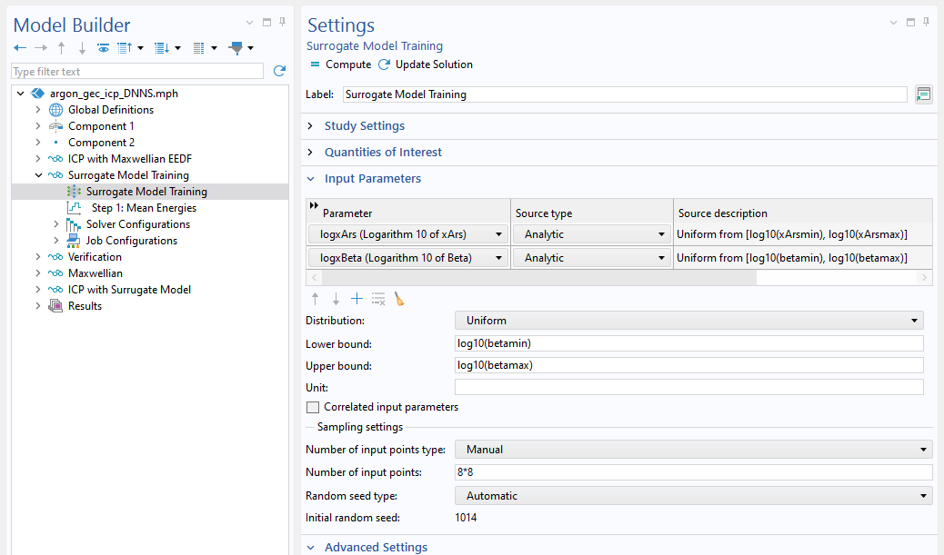 Settings of the Surrogate Model Training node showing the Input Parameters section.
Training the Deep Neural Network
After running the study with the Surrogate Model Training node, a Deep Neural Network node is automatically created under Global Definitions. This is where the actual training of the DNN occurs. Before starting the training, a few important adjustments should be made.
Enabling Log scaling under the Scaling option is essential for many quantities of interest, as they often exhibit approximately exponential growth with respect to the inputs. Applying log scaling to these outputs improves training performance by effectively balancing out errors across several orders of magnitude. Choose the Number of epochs between 10,000 and 30,000 to ensure sufficient training.
Once these settings are configured, you can click Train Model to begin training the neural network.
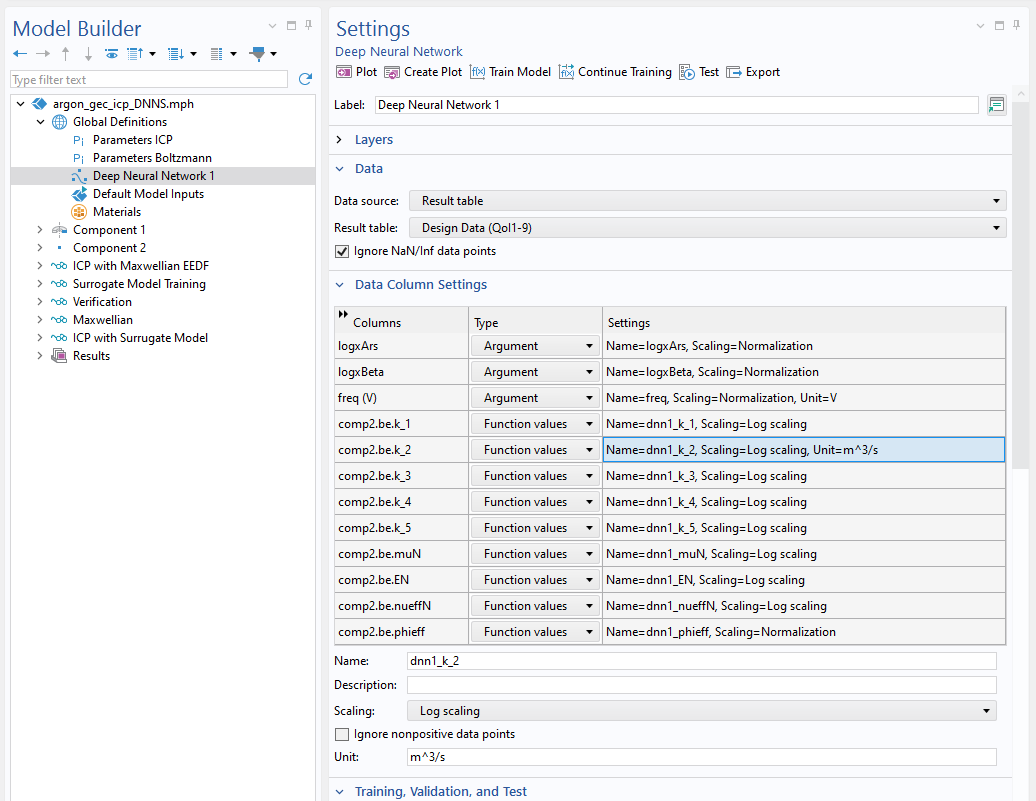 A screenshot of the Deep Neural Network node settings showing the Data Column settings.
Evaluating Quantities of Interest and Visualizing the Quality of the Fit
To visualize the neural network output, simply click the Create Plot button in the Settings window. In this example, we want to generate 1D plots as a function of the mean electron energy. To do this, modify the settings in the Plot Parameters section as shown in the figure below, then click Create Plot. This action creates a plot of the rate constant for electron impact reaction 4, with the argon excited state mole fraction and ionization degree both set to 10-6. A Grid 1D dataset is also created automatically, which can be used for further evaluations and plotting the neural network function.
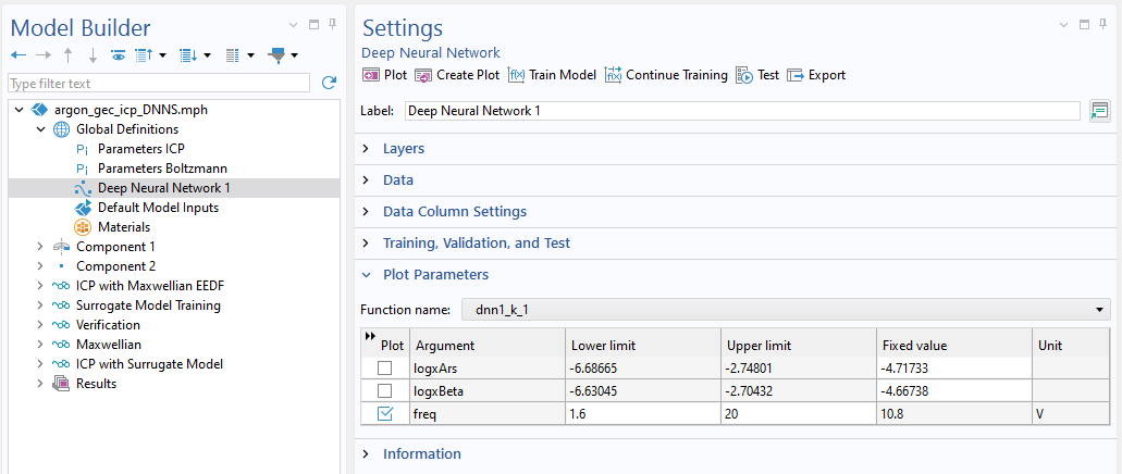 A screenshot of the Deep Neural Network node settings showing the plot parameter settings.
Each quantity of interest can be evaluated using a function name constructed from the function name defined in the Surrogate Model Training node, prefixed by the DNN name. For instance, the rate constant for electron impact reaction 4 can be evaluated using:
dnn1_k_4( Argument_1 , Argument_2, Argument_3)
where Argument_1 , Argument_2, and Argument_3 are the log10 of the argon excited state mole fraction, log10 of the ionization degree, and mean electron energy, respectively.
The figures below show a comparison between the computed data with the Boltzmann Equation, Two-Term Approximation interface and the corresponding evaluations from the trained neural network for two quantities of interest: electron mobility and ionization rate coefficient from the ground state. These results are plotted as functions of mean electron energy for xAsr = Beta = 10⁻⁶, 10⁻⁴, and 10⁻³. For reference, the values calculated assuming a Maxwellian EEDF are also included. Overall, the neural network provides a very good fit to the computed data across the parameter space.
As shown, the quantities computed with the Boltzmann Equation, Two-Term Approximation interface differ significantly from those computed using a Maxwellian distribution, particularly in the low-energy regime, where most cold plasma reactors operate. This highlights not only the importance of accurately computing the EEDF but also the significant dependence of transport and reaction rates on both the argon excited state mole fraction and ionization degree.
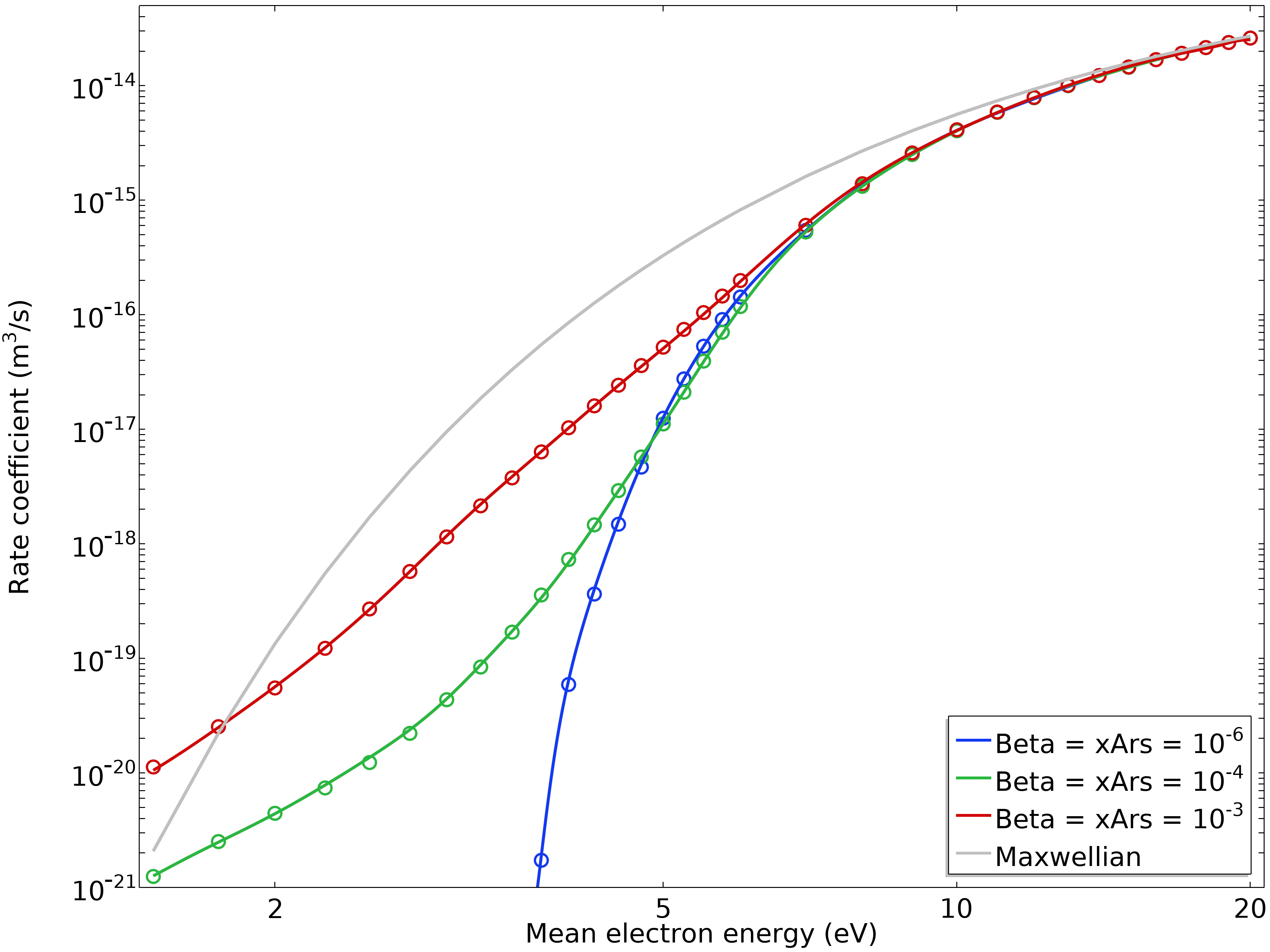 Ionization rate coefficient from the ground state as a function of the mean electron energy for a mole fraction of Ars and ionization degree equal to 10⁻⁶, 10⁻⁴, and 10⁻³. Solid lines (blue, red, and green) represent the outputs of the surrogate model and the symbols (open circles) are the data computed with the Boltzmann Equation, Two-Term Approximation interface.
 Reduced electron mobility as a function of the mean electron energy for a mole fraction of Ars and ionization degree equal to 10⁻⁶, 10⁻⁴, and 10⁻³. Solid lines (blue, red, and green) represent the outputs of the surrogate model and the symbols (open circles) are the data computed with the Boltzmann Equation, Two-Term Approximation interface.
Using DNNs in a Space-Dependent Model
To use the DNN in a spatially dependent plasma model, simply call them as functions, just as you would with any user-defined expression as shown in the figures below. In this example, we replace all electron impact rate coefficients, reduced electron mobility, effective collision frequency, and field coefficient. One important consideration is that extrapolation outside the range of the training data is generally unreliable and should not be trusted. To prevent this, we implement hard caps at the boundaries of the parametric sweep range with the following expressions:
betaSpace = log10(if(betaVar> Lmax, Lmax, if(betaVar < Lmin, Lmin, betaVar)))
xArsSpace = log10(if(plas.x_wArs > Lmax, Lmax, if(plas.x_wArs < Lmin, Lmin, plas.x_wArs)))
where Lmin = 1e-6 and Lmax = 1e-3.
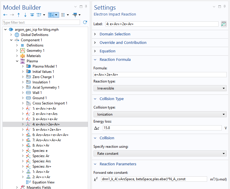 Output of the DNN used to set the rate constant for ionization from the ground state as a function of the Ars mole fraction, ionization degree, and mean electron energy.
Applying the Deep Neural Network Surrogate Model to an Inductively Coupled Plasma Reactor
In this particular case, the differences between the model results are noticeable but relatively subtle. This is because, in the bulk of the plasma, the high ionization degree tends to drive the EEDF toward a Maxwellian shape. The most significant differences appear in the electron temperature and the argon excited state number density, as shown in the figures below.
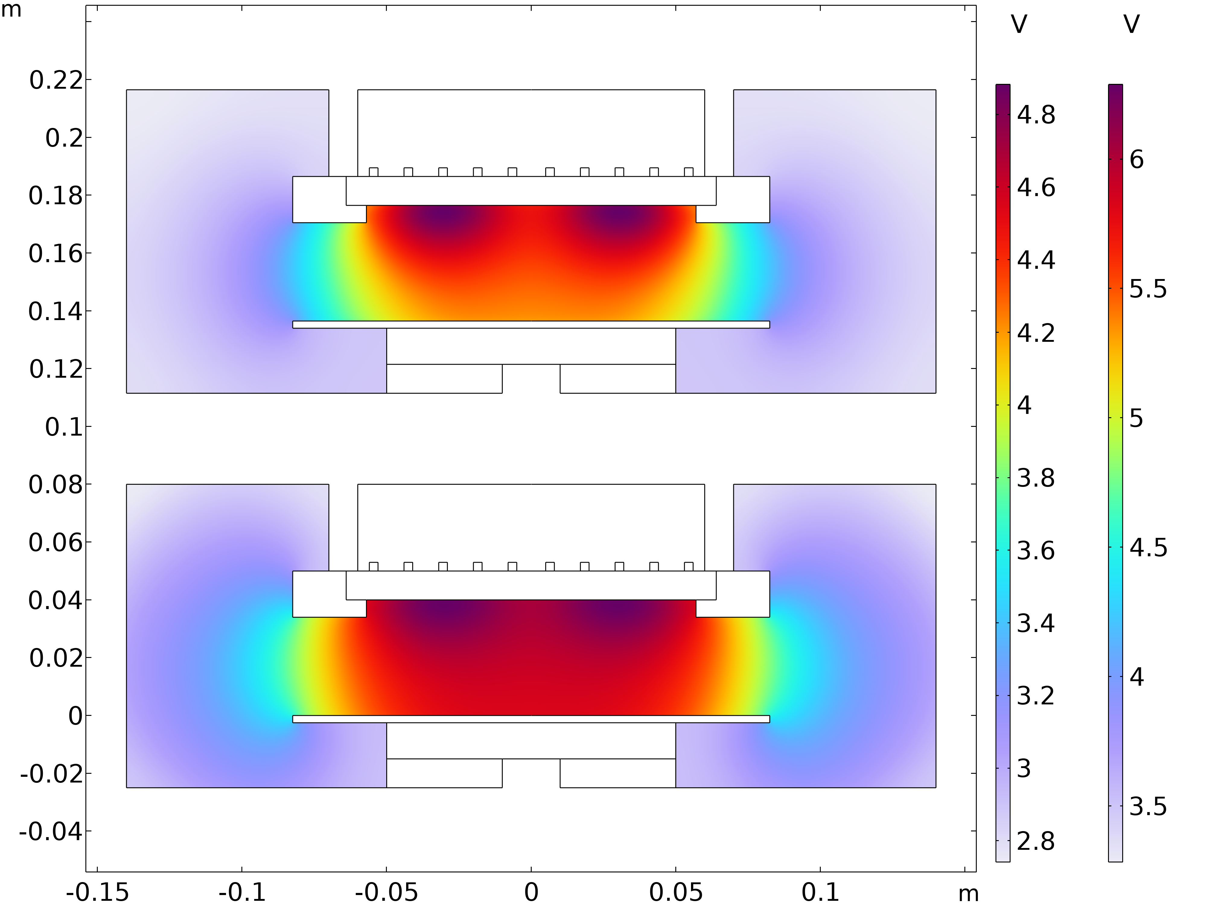 Electron temperature computed with a Maxwellian EEDF (bottom) and with the surrogate model (top).
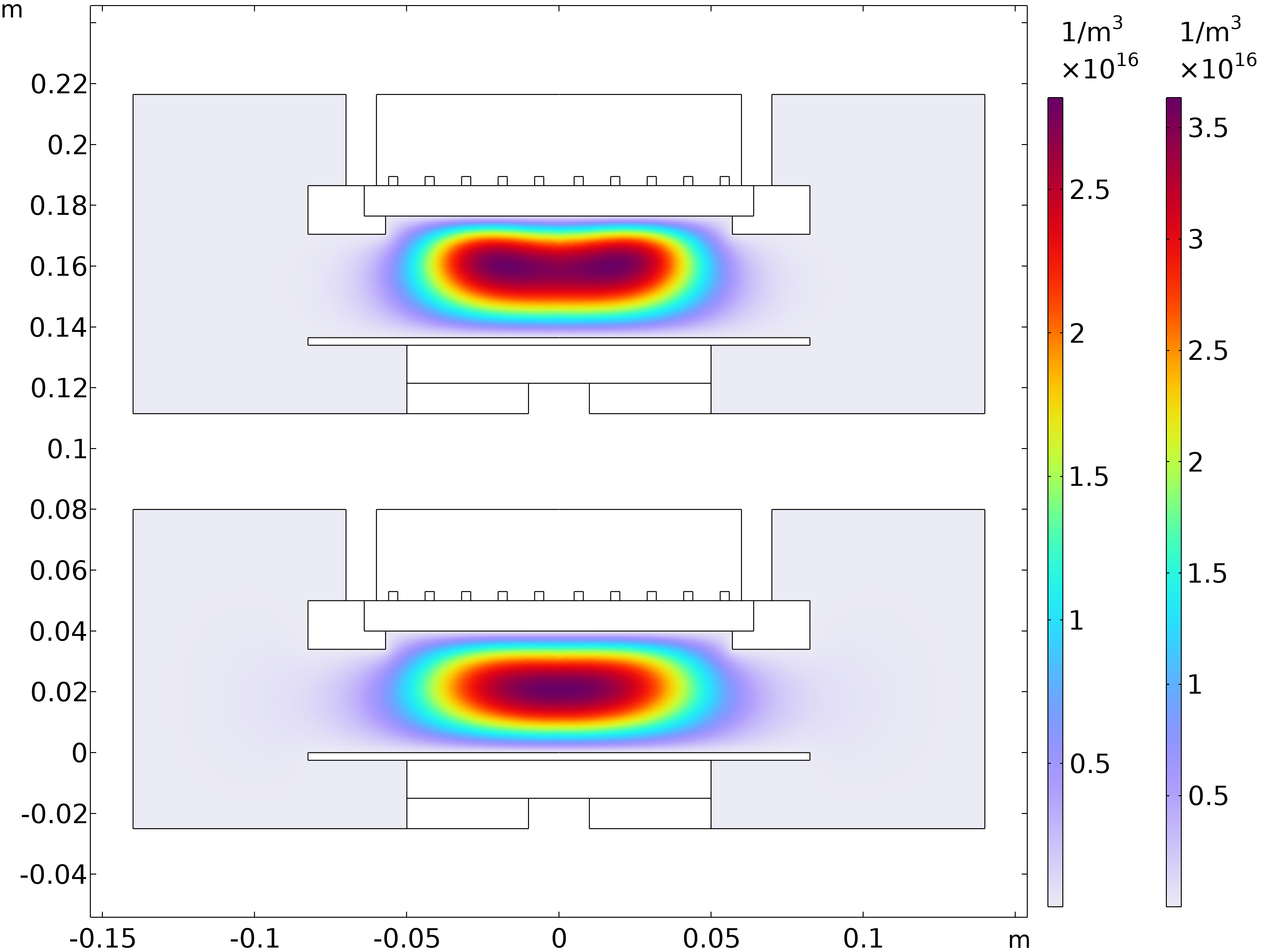 Argon excited state number density computed with a Maxwellian EEDF (bottom) and with the surrogate model (top).
Using a Maxwellian EEDF, ionization is more easily sustained, allowing the discharge to be maintained at a lower electron temperature. However, under operating conditions where the ionization degree is low, a Maxwellian assumption is likely to yield results that deviate substantially from reality. In such cases, using a more accurate EEDF becomes critical for reliable modeling.
The computational time for the ICP model using the Deep Neural Network and a time-dependent solver is approximately 10 minutes. In contrast, solving the Boltzmann equation in the two-term approximation, fully coupled with the plasma fluid model, takes on the order of an hour. This highlights the significant advantage of incorporating DNNs to introduce kinetic effects into a plasma fluid model. Even when accounting for the time required to create the data and train the DNN, the benefits remain substantial, as the DNN can be reused across various applications, effectively diluting the time cost over time. In the model featured in this blog post, we further reduce computational costs by using a stationary solver initialized with results from the model solved using the analytic EEDF. This method is highly efficient for steady-state solutions, with a computational time of just a few seconds.
Next Step
To try the example featured in this blog post, click the button below. Doing so will take you to the Application Gallery, where you can download the MPH file for the model.
Reference
- G.J.M. Hagelaar and L.C. Pitchford, “Solving the Boltzmann equation to obtain electron transport coefficients and rate coefficients for fluid models,” Plasma Sources Science and Technology, vol. 14, pp. 722–733, 2005
Comments (0)