
In a previous blog post, we introduced readers to different kinds of electron energy distribution functions (EEDFs) and their importance in plasma modeling. Today, we focus our attention on the Boltzmann Equation, Two-Term Approximation interface, demonstrating its use with an example from our Application Library.
Editor’s note: The original version of this blog post was published on April 8, 2015. It was updated on February 24, 2022, to reflect functionality available in version 6.0 of the COMSOL Multiphysics® software. Subsequently, links to the proof-of-concept model and additional learning resources were added.
An Introduction to the Boltzmann Equation, Two-Term Approximation Interface
In a plasma model, the electron energy distribution function as well as the transport properties of the electrons (e.g., electron mobility) are needed. For the simplest cases, a Maxwellian EEDF and a constant value for the electron mobility can be used. The other transport properties are then computed in COMSOL Multiphysics using Einstein’s relation. However, in some cases, it might be advantageous to use an EEDF obtained from the solution of the Boltzmann equation and define the electron transport properties as a function of the mean electron energy. But how do we obtain this data?
The answer: The Boltzmann Equation, Two-Term Approximation interface in COMSOL Multiphysics. Examples illustrating the use of this interface are available in the Application Library, one of which is the Argon Boltzmann Analysis model. To compute the Boltzmann equation in the two-term approximation, parameters such as the ionization degrees of the plasma are required. These parameters are not known a priori. Thus, the procedure is an iterative process.
The process begins with making an initial guess for the parameters and solving the Boltzmann equation. Then, the EEDF and transport properties are imported, if needed, to your plasma model. Finally, the plasma model is computed and the Boltzmann equation is re-solved with the new parameters from the plasma model. You can continue to repeat these steps until convergence is reached.
Let’s walk through the steps of creating, exporting, and importing the data into the plasma model.
Electron Energy Distribution Function and Electron Transport Properties
Create the Data from the Boltzmann Equation, Two-Term Approximation Interface
The first step is to create the data by solving the Boltzmann equation in the two-term approximation. The figure below shows a screenshot from the Boltzmann Equation, Two-Term Approximation interface used for this step. You need to define a constant Maximum energy value for the electron energy. In our example, this is set to Emax = 100 V. In addition, you need a Mean Energies study to compute the EEDF for a range of mean electron energies.
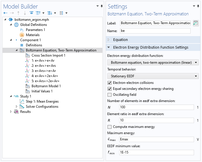
A screenshot showing the settings for the Boltzmann Equation, Two-Term Approximation interface.
The figure below shows computed EEDFs in an argon plasma for several mean electron energies. The plasma features a gas temperature of 400 K, an electron density of 1018 1/m³, an ionization degree of 10-6, and a mole fraction of excited argon of 0.01 %. It can be observed that the EEDF is a function of the electron energy.
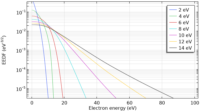
Computed EEDFs in an argon plasma.
The next figure depicts the corresponding reduced electron transport properties computed with the Boltzmann Equation, Two-Term Approximation interface. The data is a function of the mean electron energy.
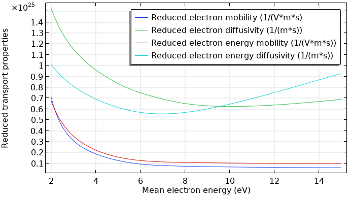
Reduced electron transport properties in an argon plasma.
Exporting the Data from the Boltzmann Equation, Two-Term Approximation Interface
The EEDF has to be imported to the plasma model as a spreadsheet consisting of three rows. The first row (x data) has to be the electron energy (eV), while the second row (y data) has to be the mean electron energy (eV). Meanwhile, the third row must contain the value for the distribution function (eV^(-3/2)). Finally, you need to export a 2D plot that looks like the following image.
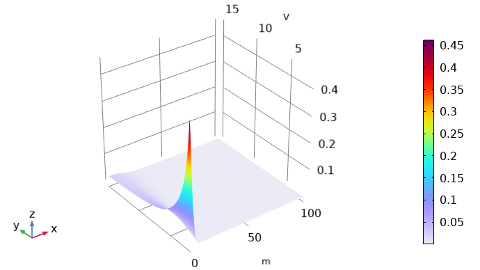
A 2D plot of the computed EEDF. Here, the x-axis indicates the electron energy and the y-axis represents the mean electron energy. The color illustrates the value of the distribution function.
Note on units: In the Plasma Module, the electron energy and electron mean energy appear with units of V but internally are treated as eV. As such, in this context, V should be read as eV. The extra dimension that represents the electron energy and on which the EEDF is solved appears with units of meters but is treated internally as eV.
To export the EEDF in the desired format, use the Parametric Extrusion dataset. The Parametric Extrusion extends the dataset with the parameter (the mean energies in this case). Right-click Datasets and choose Parametric Extrusion 1D.
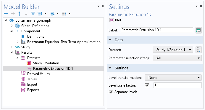
A screenshot showing the settings for the Parametric Extrusion 1D dataset.
The Boltzmann Equation, Two-Term Approximation interface is a 0D interface and uses an extra dimension to represent the electron energy on a 1D axis. As the extra dimension is normalized to the Maximum energy value, it has to be manually scaled with the Maximum energy value before exporting the data. To do this, we can use a Transformation dataset. With a Transformation dataset, you can scale, rotate, and move datasets. So right-click Datasets and choose Transformation 2D. Set the x-scale to the maximum energy (Emax in this case).
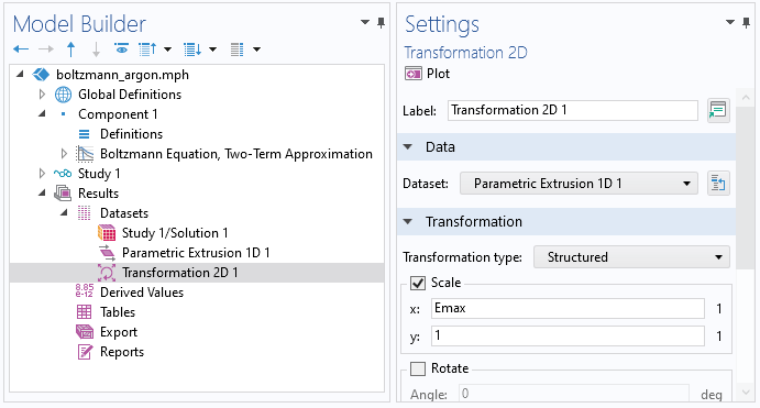
A screenshot showing the settings for the Transformation 2D dataset.
Then, right-click the Transformation 2D data and choose Add Data to Export. Enter be.f in the Expression window. Select a filename and click Export.
The transport properties can be exported in a straightforward manner from the respective 1D plot. Right-click the Global node in the 1D plot and choose Add Plot Data to Export. Select a file name and click Export.
Importing the Data to the Plasma Model
To import the EEDF to the plasma model, create an Interpolation function. Select File as the data source and enter 2 in the Number of arguments field. Click Browse and import the file.
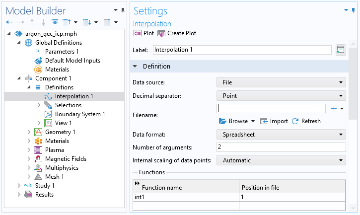
A screenshot showing the settings for the Interpolation function.
Once you have done this, you can choose the interpolation function as an EEDF in the Electron Energy Distribution Function settings in the main node of the plasma model. This is illustrated in the screenshot below.
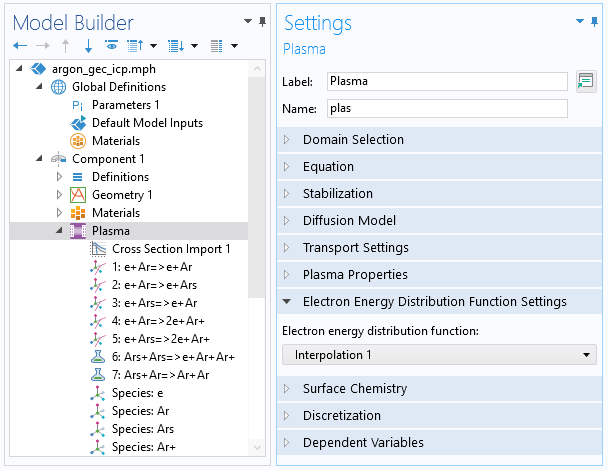
A screenshot showing the settings for the Plasma interface, which is needed to consider the precalculated EEDF.
The functions for the transport properties, such as electron mobility and diffusivity, can also be imported as an interpolation function. Here, however, the number of arguments is 1. In the plasma model node, you can use this interpolation function by entering int2(plas.ebar). In this case, int2 is the name of the function, plas is the tag of the interface, and ebar is the mean electron energy.
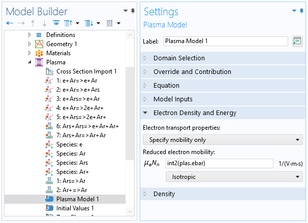
A screenshot showing the settings for the Plasma Model node, which is needed to consider the precalculated reduced electron mobility.
Next Step
Try out the approach suggested in this blog post by downloading the model of dielectric barrier discharge with different EEDFs from the Application Gallery.
Further Learning
Browse these materials related to different aspects of EEDF calculation and handling in COMSOL Multiphysics®:
- Blog post: Electron Energy Distribution Function
- Blog post: Global Modeling of a Non-Maxwellian Discharge in COMSOL®
- Tutorial model: DC Glow Discharge Coupled with the Two-Term Boltzmann Equation
You may also want to check out our blog post about different approaches implemented in COMSOL® for the modeling of different plasma types or the online course in our Learning Center devoted specifically to the modeling of nonequilibrium plasma:
- Blog post: Thermodynamic Equilibrium of Plasmas
- Learning Center course: Introduction to Nonequilibrium Plasma Modeling
Comments (4)
CHANYEOP PARK
January 14, 2016Can anyone tell me what 3 0(in the 3rd line) and 1. 1.(in the 4th line) means in the ‘collision cross section’ file for the plasma module?
EXCITATION
e+O2=>e+O2
0.1900 3 0
1. 1.
—————————
4.000000e+000 2.220446e-036
…
4.500000e+001 2.220446e-036
—————————
Pouyanesh Co.
October 14, 20203 is the statistical weight ratio and 0 means the unbalance relation between reaction and the reversed reaction.
weifeng deng
December 7, 2019请问内插函数的文件可以共享吗?
weifeng deng
December 7, 2019Can I share the file of interpolation function?