

Ferromagnetic materials are ubiquitous in electronic components and electrical machinery. In EM modeling, we may be interested in the broader application or focus on a certain material characteristic (e.g., the mechanical resistance of structural steel) that happens to be magnetic. In both cases, ferromagnetic parts influence the magnetic field in their surroundings, and identifying exactly how this happens could be crucial to the proper functioning of a device or system.
Classification of Magnetic Materials
To understand the huge variety of magnetic behaviors in different materials, classification is useful. The easiest classification system for magnetic materials is as follows:
- Weakly magnetic materials
- Slightly alter externally applied magnetic fields (i.e., paramagnetic and diamagnetic materials)
- Soft irons
- Efficiently concentrate an external magnetic flux, but don’t have an “intrinsic” magnetization (so if they are placed in a region without magnetic fields, it will remain without fields)
- Hard irons, which will be referred to from now on as permanent magnets
- Produce magnetic flux even in the absence of an externally applied field
Materials in categories 2 and 3 are referred to as ferromagnetic.
However, this classification is not simple, because the separation between soft irons and permanent magnets might not be that sharp and certain behaviors could be intermediate between the two categories. It is possible for a material to have some small magnetization in the absence of external sources (resembling a permanent magnet), but this magnetization increases by a significant amount because of an externally applied magnetic field (resembling a soft iron).
Moreover, a material can exhibit hysteretic behavior, which means that after the application and removal of an external load, the magnetization could be different from the initial one. The external load could not only be the magnetic field generated by an electric current but also a physical displacement (as shown in the video below).
When dealing with ferromagnetic materials, we may need to describe very different behaviors. In this blog post, we will analyze the options available in the COMSOL® software to do so.
Overview of Magnetic Constitutive Relations
The variety of magnetic behaviors is found (desirably or undesirably) in different systems, and being able to characterize the span of behaviors is important.
The AC/DC Module offers automatic support for including all typical magnetic behaviors via eight predefined constitutive relations, which are listed in the first column of the table below, and one option for writing your own code-based external material. Weakly magnetic materials are typically characterized by the first option, Relative permeability, which is the default in the COMSOL Multiphysics® software.
Dealing with a ferromagnetic material may require one of the other options. The first four options in the table below are tuned for soft irons and the next four are tuned for permanent magnets. Both groups are ordered in an increasing level of complexity of the constitutive relation with an increasing number of properties to describe the magnetization dynamics.
| Constitutive Relations | Soft Iron, (Fully Time-dependent) | Soft Iron (AC Feeding) | Permanent Magnets (Fully Time-Dependent) | Required Information |
|---|---|---|---|---|
| Relative Permeability | ✓ | ✓ | 1 scalar (or tensor) | |
| Magnetic Losses | ✓ | 2 scalars (or tensors) | ||
| B-H Curve | ✓ | 1 function | ||
| Effective B-H Curve* | ✓ | 1 function | ||
| Magnetization | ✓ | 1 vector | ||
| Remanent Flux Density | ✓ | 1 scalar (or tensor) and 1 vector | ||
| BH Nonlinear Permanent Magnet | ✓ | Function and a direction | ||
| Hysteresis Jiles-Atherton Model | ✓ | ✓ | 5 scalars (or tensors) | |
| External Magnetic Material** | ✓ | ✓ | ✓ | Externally compiled code |
Summary of the use of the laws to model soft or hard irons and the number of parameters to input. *For Effective B-H Curve, the function can be automatically calculated from the standard B-H curve with an example simulation app in the AC/DC Module Application Library. You can learn more about these capabilities in a previous blog post.) **External Magnetic Material is a suboption of the B-H curve. More information for this condition can be found in a blog post on accessing external material models.
In the section below, there are eight plots illustrating the typical dynamics in the B-H plane for the various constitutive relations explained in the table above. In B-H plots, the y-axis shows the magnetic flux density B. When interpreting the magnetic flux, there is not much space for ambiguity, as it is directly measurable. The x-axis is a measure of the magnetic field H. For H, the interpretation may depend on details of the analyzed system (this will be explained in an example later on).
For now, we consider an ideal magnetic circuit where the material is a torus of length L wound uniformly by a coil of N turns carrying a current I. In this case, H = N*I/L. Depending on the application, such a design (or a different one, such as an Epstein frame) may be used from the manufacturer to display B-H curves.
Here, we mention some examples of how to use these conditions in common magnetic materials, employed in some typical applications.
Laws for Soft Irons
| Constitutive Relation | B-H Behavior | Comments |
|---|---|---|
| Relative Permeability |

|
|
| Magnetic Losses |

|
|
| B-H Curve |

|
|
| Effective B-H Curve |

|
|
Laws for Permanent Magnets
| Constitutive Relation | B-H Behavior | Comments |
|---|---|---|
| Magnetization |

|
|
| Remanent Flux Density |

|
|
| BH Nonlinear Permanent Magnet |

|
|
| Hysteresis Jiles-Atherton Model |

|
|
Notice that we did not mention the external magnetic material option from the first table. This is a suboption, found by selecting the B-H Curve constitutive relation, that can be used for modeling even more general magnetic laws. A detailed example is explained in this previous blog post. This option is typically used for custom-made hysteresis models that may include conditional logic.
All of the parameters and functions discussed in the tables above can be functions of all other parameters in the model. This is extremely important, as the function can be used to include multiphysics effects or to have extra freedom in handling material nonlinearities.
An example where a nonlinear dependency is added manually to the Relative Permeability case so that it can behave exactly as the B-H Curve case is featured in a tutorial model on the topology optimization of a magnetic circuit. The example shows that transforming the case is as easy as writing in the field for relative permeability: murOfB(mf.normB). This is useful because the permeability is then set to: 1-p^2+p^2*murOfB(mf.normB), so that the law is describing air in the region where p is 0, and a soft iron in the regions where p is 1. (In the model, p is a function varying according to a topological optimization. Notice that, as is explained in the model documentation, writing a function of normB could also require other actions in order to avoid convergence issues. In the model, the option “Split complex variables in real and imaginary parts” was activated.)
Induction heating is another useful application for setting permeability as a function. In these cases, the material is crossing the Curie temperature. This is commonly done by means of setting a permeability to a function of the form 1+f(T)*(mur(normB)-1), where f(T) is a function that decreases from unity at low temperatures to 0 at the Curie temperature (remaining at 0 above that temperature). This method is needed to accurately model many induction heating processes of steels (e.g., hardening). More generally, many functional dependencies of BH parameters versus temperature can be retrieved from either literature or data sheets, and we can insert them using the same method.
Many parameters, even if referred to as “scalar” or “function” in the table, can be “tensors” or a set of functions filling a vector or a tensor. This is important because magnetism is intrinsically vectorial in nature. In fact, for all of the described behaviors in the first table, the AC/DC Module gives us the option to model completely anisotropic materials. Such an example is discussed in this tutorial model on vector hysteresis, where an anisotropic Jiles-Atherton material is used and reproduces published data.
The vectorial nature of fields is crucial for modeling moving magnetic machines. The animation below shows the magnetic flux density in a rotating machinery simulation where the outer domain is described according to a Jiles-Atherton hysteresis model. On the left, the hysteretic domain rotates, and on the right, the inner magnet rotates. Comparing any point in the left image with the corresponding point in the right image, all components of the vectors B and H follow the transformation that vectors must satisfy due to rotation. This results in the animation on the right being a rigid rotation of the animation on the left.
Magnetic flux for rotating machinery, including a hysteretic material showing that the vector nature is exact so that the local fields are identical both in the frame of the magnetic field source (left) and in that of the hysteretic domain (right).
Modeling Ferromagnetic Materials Using COMSOL Multiphysics®
Next, let’s consider an example that shows that different laws can be used for the same piece of ferromagnetic material when modeling its behavior during different processes. This is given that only a limited set of typically retrievable material information is available.
Here, we model a magnetic circuit, depicted in the figure below. The red part is a nonlinear soft iron piece characterized by no significant remanent flux and a hysteretic B-H curve (from the Soft Iron material available in AC/DC Module Material Library: knee reaching 1.5[T] at about 5400[A/m]). The blue domains represent a coil that is wound around the soft iron core. The green domain is the piece of interest, which we analyze using different laws. This could be an AlNiCo component that is initially not magnetized.
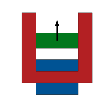
Geometry of the magnetic circuit, featuring soft iron (red); a coil (blue); and an AlNiCo-like material (green). The AlNiCo bar is initially nonmagnetic, then magnetized because of an applied current to the coil and demagnetized because of the extraction from the magnetic circuit (arrow).
We can simulate the magnetic circuit in four different working conditions:
- The AlNiCo component starts from a nonmagnetized state and magnetizes because of an applied current to the coil
- The AlNiCo component is magnetized because of the current of Step 1 and keeps most of its magnetization, even when the coil current is removed
- The magnetized AlNiCo component at the end of Step 2 gets partially demagnetized when extracted from the core
- The demagnetized AlNiCo component is brought back in the magnetic circuit, essentially keeping the low magnetic remanent flux from when it was out of the magnetic circuit
We may be tempted to tune the constitutive relation for the whole cycle. This is indeed possible, but usually requires specific independent measurements from the iron manufacturer. For example, it could be easy to know the value of H where the material can be considered as fully magnetized, the corresponding remanent flux, and the demagnetizing curve.
For the current example, let’s say that we know that saturation is reached for an externally applied magnetic field of 30[kA/m] and that the (uniaxial) demagnetization curve in the second quadrant of the B-H plane is reported in the table below. The curve starts at the remanent flux Br at H = 0 and approaches B = 0 at the (negative) coercive field Hc. Notice that the data reported in the table exactly represents the material you will find in COMSOL Multiphysics by selecting Demagnetizable Nonlinear Permanent Magnet under the AC/DC Module Material Library.
If you wish to import your own data, take a look at the embedded example material. Notice that you will need to provide the coercive magnetic field Hc and a properly placed demagnetization curve. Given the original curve spans the second quadrant, the curve should be translated along the H-axis by abs(Hc). When doing so, the input B-H curve will start at (0,0) and reach the remanent flux density Br at the value abs(Hc). Further instructions can be found in the AC/DC Module User’s Guide.
| H [kA/m] | B [T] |
|---|---|
| -50 (coercive magnetic field, Hc) | 0 |
| -48 | 0.5 |
| -47 | 0.7 |
| -46 | 0.85 |
| -44 | 0.96 |
| -40 | 1.03 |
| -35 | 1.08 |
| -30 | 1.11 |
| -20 | 1.155 |
| -10 | 1.187 |
| 0 | 1.2 (Remanent flux, Br) |
Data for the second quadrant B-H curve of the Demagnetizable Nonlinear Permanent Magnet material available in the AC/DC Module Material Library.
The trajectory of the horizontal component of magnetic flux density in the center of the AlNiCo component during the four-part processes is depicted in the image below. The colors represent the following stages:
- Blue curve: relative to current feeding (this step of the process starts from left at H = 0, no current; reaches a maximum magnetization at far right)
- Green curve: relative to the process of removing current (starting on the far right; reaching a finite magnetic flux density on the left H = 0 level, where no current is flowing in the coil)
- Red curve: relative to the demagnetization process due to the extraction from the magnetic circuit; exactly follows the data of the table above
- Cyan curve: reinsertion of the magnet in circuit; the process starts on the left (object completely out of the circuit) and ends on the right (object fully inside the magnetic circuit)
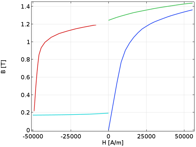
Horizontal component of magnetic flux density in the center of the AlNiCo during the four-step process.
The video below shows the conditions that have been applied to the AlNiCo component and result in the trajectory of the graph above.
Notice that all of these simulations are very easy and robust parametric stationary simulations, which are eventually starting from the previous solution. With such a setup, developing the same model in 3D or with more complex geometries would have been just as easy. As we commented before, we have used previous solution data to connect behaviors in different regions. This is the origin of the small discontinuities that are shown in the curve of the graph above.
The model can be adapted to make the process exactly continuous, but distinguishing eventual extra parameters would likely require extra information and measurements. By following this procedure, we have shown that such measurements may not be that compulsory and that reasonable solutions can be found using the material data that is typically available.
When looking at the hysteresis loop of the graph above, we should make a note regarding the quantity that is read on the x-axis. During Steps 1 and 2 on the x-axis, it is natural to read a quantity that is proportional to the driving current. During Steps 3 and 4, there is no current in the coil and the fields depend on the component’s spatial displacement. So it is not easy to unambiguously decide the quantity to be used on the x-axis. In Step 3, we use a built-in variable, called axialH. In Step 4, we use a normalized displacement from the circuit. These differing definitions are important when reading a B-H curve to be sure of the researcher’s intentions (i.e., which experimental apparatus was used) when creating graphs.
In this example, we have shown that we can alternate different constitutive relations in different studies and that, in the properties of these constitutive relations, we can write any expression depending on variables computed in previous solutions. Here, we did so in the most simple way in order to avoid overcomplicating the discussion. For a more advanced and rigorous 3D model of AlNiCo extraction and reinsertion in a magnetic circuit, you can check out this self-demagnetization model. There, a local linear recoil model for magnet reinsertion is added.
Conclusion
In this blog post, we have analyzed the wide variety of options present in COMSOL Multiphysics and the AC/DC Module for modeling magnetic materials. We started with the basic principles of magnetism and the suite of conditions that are offered, pointing to actual materials and devices for which each available law is more appropriate. We have also commented on the functionality for multiphysics modeling and implementation of more advanced conditions.
That said, we only covered a margin of the important aspects that are taken into account when deciding a constitutive law. We invite you to refer to the additional resources below and to contact us for more information about the software.
Next Steps
Get an overview of the capabilities of the AC/DC Module for modeling magnetic materials and more. If you would like to see the software in action, you can request a demonstration from the product page.
Additional Resources
- Watch an archived webinar on ferromagnetic modeling concepts
- Check out these related blog posts:
- Try these tutorial models:


Comments (11)
João Silva
October 29, 2018Hello Cesare
I can’t find the 2D model of the moving AlNiCo bar in the gallery.
Can it be made available?
Thanks in advance
João
kevin mckinstry
December 7, 2018A permeameter of sorts can be made by adding a coil to the soft yoke structure here. If this is done and current is applied to the coil to drive the AlNiCo sample past saturation in both directions, will it result in a fair representation of the sample’s hysteresis curve?
Cesare Tozzo
December 11, 2018 COMSOL EmployeeInteresting comment/request Kevin! Yes, we have different option to achieve what you ask. I even just prepared a small model using “Nonlinear Permanent Magnet” constitutive relation (using two different curves for different paths) and it seems to work! Thank you for inspiring me about this alternative that it is something that I wanted to test at a certain point, but I think I did not really tried! If you contact support, we can help you understanding the best alternative for your specific case and share relevant models.
João, the same applies for you. Please contact support and we will let you have relevant models that can help you (btw, the extraction part of the 2D model is essentially identical to the 3D case which is linked in the page and you can download by a COMSOL acceess – the other part of the process use different studies that activate different features, eventually linking with solution from other models).
Support email: support@comsol.com
David Xu
April 4, 20191) Can COMSOL simulate stress induced magnetization of carbon steel pipe in earth magnetic field.
The fundamental physics is the well-known Villari Effect—- the domain structure of a ferromagnetic, which determines its magnetic properties, changes when mechanical force is applied.
2) stress-strain distribution of the defects in pipe can be very well simulated and provided as inputs. Carbon steel material stress-strain curves will be provided as well.
3) How COMSOL can simulate the resulted magnetization? Plastic stress/strain and elastic stress/strain have different effects. Can COMSOL handle the two different cases? Magnetoelasticity vs magnetoplasticity.
4) What are the required inputs and what are the outputs?
Cesare Tozzo
April 5, 2019 COMSOL Employee(For David Xu and all reader interested in similar topics) COMSOL has an automatic support for magnetostriction. Once the coupled magneto & elastic constitutive relations are known, you have different ways to make the material behave as you desire. Specific implementations in your case may depend on the details of the material.
In this context, the best is that you to refer to support@comsol.com and your COMSOL Representative.
For introductory information about some of the options offered by COMSOL for magnetostriction, these are useful reading
* https://www.comsol.com/blogs/etrema-analyzes-magnetostrictive-materials-with-simulation/
* https://www.comsol.com/model/nonlinear-magnetostrictive-transducer-6063
* pages from 412 to 419 of “Structural Mechanics Module, User’s Guide” (pages refer to version 5.4) that is shipped within COMSOL installation
Magnetostriction requires the AC/DC Module and one of the Structural Mechanics Module, MEMS Module, or Acoustics Module (see https://www.comsol.com/products/specifications)
Salvatore Circosta
June 19, 2019Hello Cesare,
very interesting post!
I am currently working on the simulation of a magnetic hysteresis machine in Comsol Multiphysics 5.3. When feeding the stator with a three-phase current set, the hysteresis torque seems to match well what we measured in our lab. However, when applying the moving mesh, the torque is substantially larger than what we measured (in some cases it doubles what we expect). We are suspecting that the moving mesh and the vector Jiles-Atherton model are somehow interacting. Any ideas?
Thanks in advance,
Salvatore
Cesare Tozzo
December 9, 2019 COMSOL EmployeeOn this blog I got today a question on which model was using the here described approach to model Curie Temperature effect; here it is
https://www.comsol.com/model/induction-heating-of-a-moving-ferromagnetic-mechanical-part-51821
Best regards
Cesare
Sina Jafarzadeh
June 10, 2021Relative Permeability can be considered as a function of temperature and the magnetic field while working in a low field and with a soft magnet, around and far from curie temperature. Have you considered both variables in any simulation?
How we can study both parameters?
Best
Sina
Cesare Tozzo
June 11, 2021 COMSOL EmployeeDear Sina, in the link of the comment here above ( https://www.comsol.com/model/induction-heating-of-a-moving-ferromagnetic-mechanical-part-51821 ) there is such an example including both dependencies from magnetic field and temperature (for including both Curie temperature and saturation at low temperatures). Feel free to contact us via support@comsol.com for any model specific help !
Kader Akyildirim
September 9, 2025I’m currently working on the magnetic shielding properties of superconducting tubes coated with ferromagnetic material. Do you have any research or other work I can use on this topic? Thanks in advance for your help.
Cesare Tozzo
September 9, 2025 COMSOL EmployeeKey for modeling superconductors is typically more about choosing the proper formulation, rather than just the constitutive relation. Yes, we have material that we can send contacting us at support@comsol.com