

In a previous blog post, we introduced various physical phenomena that cause damping in structures and showed how such damping can be represented mathematically. Today, we follow up by looking at how to actually include damping in finite element models.
How to Consider Damping in Finite Element Analysis
When performing a structural dynamics analysis, modeling the damping can be an important, and difficult, part of the task.
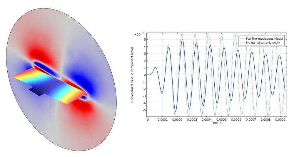
A transient analysis of a vibroacoustic micromirror, with viscous and thermal damping taken into account.
Below, you’ll find an overview of what to take into consideration when modeling damping effects in your finite element analyses with the COMSOL Multiphysics® software.
Eigenfrequency Analysis
An eigenfrequency problem can be solved with or without damping in COMSOL Multiphysics. As long as there are any dissipative effects in your model, these will be taken into account, and the computed eigenfrequencies will be complex-valued. This is automatic, so you do not need to add any special settings in the solver.
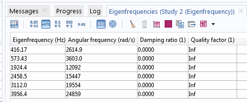
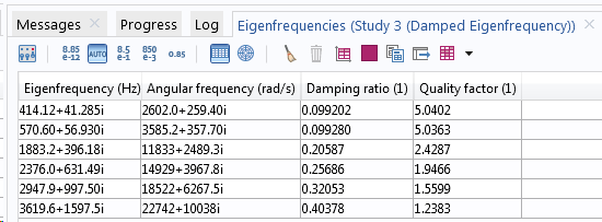
Eigenfrequencies in a model without (upper table) and with (lower table) damping.
In most cases, not only the eigenfrequencies but also the eigenmodes are complex-valued when damping is involved. The interpretation of a complex-valued mode shape is that the phase angle provides information about the phase shift between different points in the structure under free vibrations. That is, if the displacements in two points have different phase angles, they will not reach their peak values simultaneously.
In most cases, the effects of damping on mode shapes and eigenfrequencies are marginal. The main reason to include damping in an eigenfrequency analysis is to estimate how much different resonances will be damped.
Frequency-Response Analysis
If the excitation frequency is in the vicinity of a natural frequency (say within ±50%), the damping model is of paramount importance, as shown in the response curves in the previous blog post. This is a case where you really have to spend some effort on obtaining appropriate values of the damping. Close to the resonance, the results are completely controlled by the damping, so choosing between a loss factor of 0.01 or 0.02 can, in the end, mean a factor of 2 in a stress prediction.
Time-Domain Analysis
In a time-domain analysis, the damping will, in most cases, have a limited impact on the results. The exceptions are when simulating wave propagation or if the time history of the loads is such that some resonances are strongly excited.
There is, however, another important aspect of damping in time-domain analysis: It can stabilize the time stepping. It is common that spurious, less-interesting waves are generated in the structure. Unless they are properly suppressed, the time steps may become unnecessary small. To suppress such waves, it is advantageous to introduce a damping model that mainly provides significant damping at high frequencies.
Response Spectrum Analysis
In response spectrum analysis, the damping is part of the design response spectrum, so it should not be explicitly modeled. A single damping value is used to represent the whole structure.
Numerical Models for Damping
The Finite Element Formulation
In matrix form, the finite-element-discretized equations of motion can be written as
where M is the mass matrix, C is the viscous damping matrix, K is the stiffness matrix, u is the displacement vector, and the right-hand side consists of the force vector f.
The mass and stiffness matrices are computed given the geometry and basic material parameters, such as mass density and Young’s modulus. The damping matrix can, however, be formed in many different ways. Different types of damping contributions can often also be combined.
In the frequency domain, where it is assumed that the excitation and response are harmonic, the corresponding equation is
Here, the displacement and force vectors are complex-valued.
Loss Factor Damping
Loss factor damping is the primary method for describing losses in the material in a frequency-domain analysis. The mathematical description is, as discussed in the previous blog post, by a complex-valued multiplier to the stiffness.
In COMSOL Multiphysics, you can include loss factor damping through the Damping subnode under a material model. For the Linear Elastic Material, you can even give individual loss factors for the different elements in the constitutive matrix.
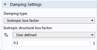
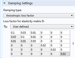
Entering loss factor damping values.
In reality, it is common that the loss factor has some frequency dependency. In a frequency-response analysis, this can be readily incorporated by making the loss factor a function of the built-in variable freq. You can either use an expression, as shown below, or reference any type of function of the frequency.
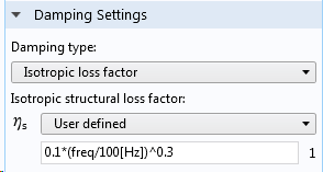
Frequency-dependent loss factor.
To see how loss factor damping enters the system of equations, assume that the same loss factor is used everywhere. Then, the damping matrix can be identified as
The equation of motion then becomes
Viscous Damping
In a viscous damping model, stresses proportional to the strain rate appear in the solid material. In the most general case, the constitutive tensor relating the stress to the strain rate can contain 21 independent constants. Since damping is difficult to measure and quantify, these values would seldom be known, and it is more common to work with isotropic viscous damping models.
Viscous damping in the Solid Mechanics interface in COMSOL Multiphysics uses two constants:
- Bulk viscosity, \eta_b
- Shear viscosity, \eta_v
The former provides a damping proportional to volume change, and the latter to shape change.
The viscous stress tensor can be written as
where \epsilon_v is the volumetric strain and {\boldsymbol \epsilon}_d is the deviatoric part of the strain tensor.
Since the damping stress is proportional to the strain rate, it will be more prominent at higher frequencies.
Viscous damping is another option in the Damping node.
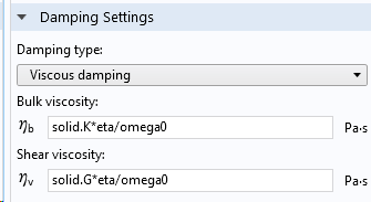
Entering viscous damping.
Viscous damping can be used in any dynamic study type.
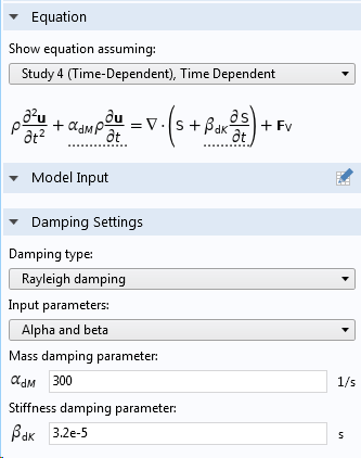
Rayleigh Damping
Rayleigh damping is a simple way of generating a damping matrix as a pure linear combination of the mass and stiffness matrices,
This damping model does not have a direct connection to physical damping processes. Originally, it was introduced because it gives a damping matrix that can be diagonalized by the eigenmodes from the undamped eigenfrequency problem, thus giving a complete dynamic decoupling between the different modes.
The stiffness matrix term (“beta damping”) can, however, be interpreted as being directly proportional to the strain rate. Actually, a pure beta damping corresponds to a viscous damping with
where K and G are the elastic bulk and shear moduli, respectively.
Beta damping, just as viscous damping, provides a damping that is stronger at higher frequencies. The mass proportional term α, on the contrary, provides a damping that is strong at low frequencies. It acts on the velocity of the structure, so it will damp a rigid body motion.
Rayleigh damping is also given in the Damping subnode under a material model. This design actually provides the freedom to create a type of damping that is a generalization of the original Rayleigh damping. In order for the damping matrix to be a linear combination of the mass and damping matrices at the system level, the Rayleigh damping parameters must be the same in all Damping nodes. If not, this property is true only at the element level.
There are two ways in which you can provide the Rayleigh damping parameters, either as a direct input of α and β or by providing the damping ratio at two different frequencies.
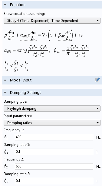
Entering Rayleigh damping in a Damping subnode to a material model.
Dissipative Material Models
Some material models contain an inherent dissipation. In this context, the most interesting case is probably viscoelasticity. When you use such material model, it will usually provide significant damping. You would, in most cases, not combine it with a Damping node on the same domain.
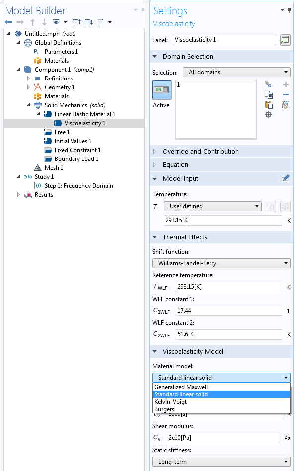
Selecting a viscoelastic material model.
Thermoelastic Damping
Thermoelastic damping can be directly incorporated into a model through a setting in the Thermal Expansion multiphysics coupling.
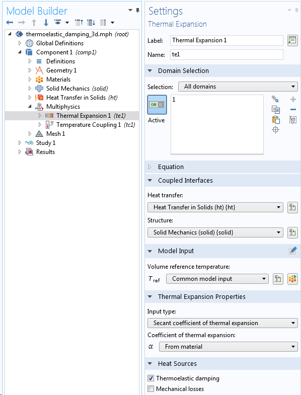
Thermoelastic damping in a coupled heat transfer and structural analysis.
The effect of including thermoelastic damping is that a heat source term, proportional to the rate of stress change, is added to the heat balance equations,
Here, T is the temperature, \boldsymbol \sigma is the stress tensor, and \boldsymbol \alpha is the coefficient of thermal expansion tensor.
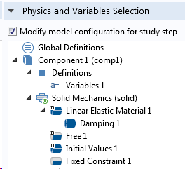
Modal Damping
Solving linear structural dynamics problems using mode superposition is a very efficient technique. When using mode superposition together with damping, there are certain things to note.
The initial eigenfrequency analysis should be performed using the undamped problem, and the damping is then included only during the mode superposition step. The most convenient way of ensuring this is through the Physics and Variables Selection section in the settings for each study step.
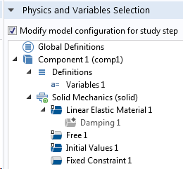
Study step settings for the eigenfrequency study (left) and subsequent mode superposition study (right).
All types of damping contributions are allowed in the mode superposition. This may not sound surprising, but it is an effect of the fact that the eigenmodes are not assumed to be decoupled in the modal solvers in COMSOL Multiphysics. This means that you can solve a wider range of damped problems than in many other implementations of a mode superposition method.
In addition to damping provided by various physics features, you can also provide a damping ratio for each eigenmode: so-called modal damping. Modal damping is particularly useful if you know from experience that some modes are more heavily damped than others. This is the case when different physical phenomena are connected to the mode shapes. Modal damping is given directly in the settings for the modal solver.
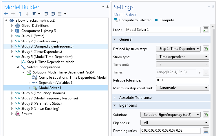
Entering modal damping.
Modal damping is added to any other damping contributions.
Infinity Boundary Conditions
When you need to model losses due to acoustic emission or anchor losses, the important thing is to equip your model with boundary conditions that allow outgoing waves to disappear without reflection. COMSOL Multiphysics offers several options here, depending on the involved physics interfaces and whether the analysis is in the time domain or frequency domain.
In the frequency domain, a perfectly matched layer (PML) is a good alternative for a boundary condition toward “infinity”. The PML formulation, which is available for many different physics interfaces, essentially attenuates outgoing waves so that the reflected energy is very small. The effect is that damping will be present in the analysis, since the energy in the outgoing waves is lost.
A PML is modeled using a few layers of elements on the exterior of the computational domain.
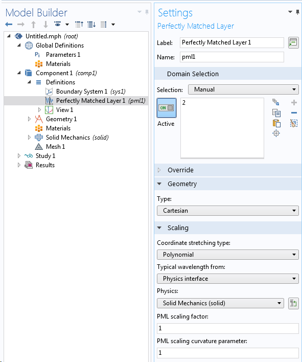
Defining a domain as a PML.
In the Solid Mechanics interface, you also can find a special type of boundary condition called a Low-Reflecting Boundary. Its purpose is the same as for the PML: to avoid wave reflection. Although it is not as efficient as a PML when the waves strike the boundaries at oblique angles, the Low-Reflecting Boundary node has two advantages:
- It can be used in time-domain analyses
- Since it is a boundary condition, it does not require extra domains to be meshed outside of the computational domain
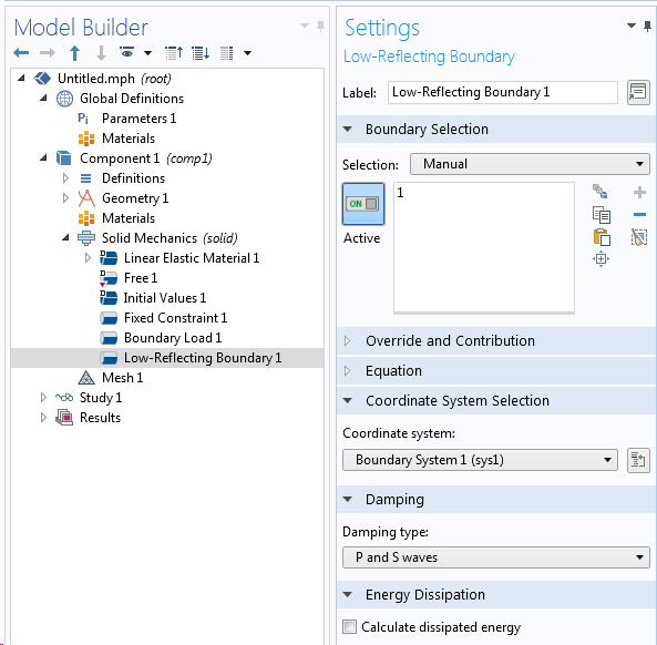
The Low-Reflecting Boundary node.
Another way of simulating waves traveling toward infinity is by using the boundary element method (BEM) formulation for acoustic waves.
Friction Between Sliding Surfaces
If friction is an important source of damping, you will often have to make some engineering approximations. In principle, you can, of course, solve a time-dependent problem with full contact modeling including friction. Unfortunately, in the vast majority of cases, this will be prohibitively expensive in terms of computer resources.
An alternative is to replace the contact zone by a thin elastic layer and equip it with viscous or loss factor damping. The problem, however, is how to estimate the shear stiffness and corresponding loss factor. General methods for estimating these parameters is a topic for recent and ongoing research. You may have to do initial local analyses of the joint to investigate its properties.
Damping in Other Features
There are many other features beyond the material models through which you can supply damping in your model. Some examples include:
- Spring Foundation feature
- Thin Elastic Layer feature
- Spring-Damper feature
- Joints and gears in the Multibody Dynamics interface
- Damper and Impedance features in the Lumped Mechanical System interface
- Bearings in the Rotordynamics and Multibody Dynamics interfaces
- Any load that is entered as velocity dependent
- Complex-valued material data
Concluding Remarks
Modeling damping in structural dynamics is an essential and nontrivial part of the model definition. COMSOL Multiphysics provides you with a broad range of options for describing damping. Obtaining the correct data for the materials and components in a structure is, however, often challenging.
Next Steps
Learn about the Structural Mechanics Module, which includes specialized features and functionality available for modeling damping:
- Read Part 1 of this blog series: Damping in Structural Dynamics: Theory and Sources
- If you are interested in modeling damping, you can find several examples showing different approaches in the Application Gallery:
- Static and Eigenfrequency Analyses of an Elbow Bracket
- Viscoelastic Structural Damper — Transient Analysis
- Bracket — Transient Analysis (bracket_frequency.mph)
- Wave Propagation in Rock Under Blast Loads
- Piezoelectric Tonpilz Transducer
- Thermoelastic Damping in a MEMS Resonator
- Disc Resonator Anchor Losses
- Vibrating Micromirror with Viscous and Thermal Damping: Transient Behavior


Comments (11)
Christopher Hoen
March 16, 2019A very good post on damping in structural systems. The content of the post should be a part of any basic course in structural dynamics. Especially the description of how to interpret complex valued mode shapes is well formulated:
“The interpretation of a complex-valued mode shape is that the phase angle provides information about the phase shift between different points in the structure under free vibrations. That is, if the displacements in two points have different phase angles, they will not reach their peak values simultaneously.”
Why it is like that is shown in my paper “An Engineering Interpretation of the Complex Eigensolution of Linear Dynamic Systems”
see
https://www.researchgate.net/publication/237658147_An_Engineering_Interpretation_of_the_Complex_Eigensolution_of_Linear_Dynamic_Systems
Henrik Sönnerlind
March 18, 2019 COMSOL EmployeeHi Christopher,
Thank you for the nice comment, and also for the interesting link.
Regards,
Henrik
Robert Gustavsson
March 18, 2019Hi! The section about damping in material models (viscoelasticity) makes me wonder. If the model is dissipative so that energy is lost, is it possible for the material to remain elastic? i.e. unloading by going along the loading path in reversed direction (sigma-epsilon plot). My spontanoues guess it that damping will make it take a different path when unloading. Maybe leave a plastic deformation as well.
Henrik Sönnerlind
March 18, 2019 COMSOL EmployeeHi Robert,
To some extent, the answer depends on how we define ‘viscoelastic’. However, the more common viscoelastic models like Maxwell, Generalized Maxwell, Kelvin-Voigt, Standard Linear Solid, etc. share the property that they, in the low strain rate limit, approach a pure linear elastic material. So when unloaded, there are no remanent strains. During dynamic cycling, the stresses and strains will however be out-of-phase, so that there is a hysteresis loop in the stress-strain diagram; hence the energy dissipation. If you define ‘elastic’ as following the same path up and down also under high strain rates, these material models do not have that property.
Other time dependent material models (that I would prefer to denote as creep or viscoplasticity) will for sure act more as plasticity and there will be remanent strains after unloading. Typical creeping materials does however have completely different time scales, so that they have low damping in a structural dynamics context.
Finally, an elastoplastic material will dissipate energy during the parts of the loading history when plastic strains are produced. Depending on the type of hardening (isotropic/kinematic) and strain levels, the material may or may not be a source of dissipation during vibration. Often, plastic strains are only produced during the first cycle. If not, we can expect the material to break from low cycle fatigue rather soon.
Regards,
Henrik
Ivar KJELBERG
March 20, 2019Hello Henrik,
Thanks for a very nice post.
I remain with a question I could not find hereby: “complex material properties”,
are these considered. In particular for a PZT material, I have found some articles that give me complex PZT properties to take into account the PZT natural damping, these are obtained from measurements on PZT material.
See i.e. http://www.norskfysikk.no/nfs/faggrupper/akustikk2011/papers/SSPA2011_AmundsenOernulf_etal__Generalised_permittivity_19p.pdf
But does COMSOL take these correctly into account, I see some damping in my models when using these complex material properties, but how to correlate and be sure it’s “correct”.
I need some calibration means, or some confirmations from the COMSOL developers, I believe.
Any comment here ?
Thanks in advance
Ivar
Henrik Sönnerlind
March 20, 2019 COMSOL EmployeeHi Ivar,
Complex notation is only meaningful in frequency domain. But there, using complex valued material data is equivalent to using loss factor damping. The loss factor damping is just a multiplication of the stiffness by (1+i*eta).
When working with piezoelectric materials like PZT, you must however be careful to use the correct sign of the imaginary part if you consider the damping as represented by complex material properties. There are some subtleties there, which in the user’s guide are explained in the section about loss factor damping in piezo materials.
Note also that built-in dissipation variables may not always capture complex valued inputs. Contributions to such variables may be generated from a Damping (or similar) subnode which is bypassed when instead of explicit damping using complex valued material data. But in most cases, also this will work.
Regards,
Henrik
Vahid Khoshkava
April 12, 2019This is the topic that I was looking for a long time. Thank you for the great material.
I have a resonating system and I am running a time domain study. Using the experimental data, I can calculate the damping factor and thus provide the loss factor value in the time domain study, but I do not see any decaying behaviour and it seems that the structure keeps oscillating even if the external force is zero (no decaying behaviour). In other words, as you mentioned correctly, the time domain behaviour (at least in my case) is not sensitive to damping ratio.
My question:
What is the proper way of defining the damping factor in the time domain study? Or what should we do to make the time domain study to be sensitive to damping to be able to compare it with experimental data?
Thanks,
Vahid
Henrik Sönnerlind
April 12, 2019 COMSOL EmployeeHi Vahid,
The fact that loss factors are only defined in frequency domain is a fundamental problem. The loss factor assumption makes the damping force proportional to displacement, rather than to the velocity. This property is not easy to replicate in time domain.
If the frequency content of your time signal is limited, you can use viscous (or Rayleigh) damping tuned to match the loss factor damping at a characteristic frequency.
Below is a link to a paper suggesting a method for implementing a better damping model for time domain, but it is difficult for a general 3D case.
https://www.researchgate.net/publication/318379818_On_strain-rate_independent_damping_in_continuum_mechanics
Regards,
Henrik
Vahid Khoshkava
April 12, 2019Thanks for the reply and valuable information.
The damping ration of the system is almost constant (over the frequency of interest); I have tried Rayleigh but did not work, unless playing with those values which becomes curve fitting rather than a modelling analysis 🙂
Is there any relation between the viscous damping and damping ratio?
Thanks,
Vahid
Henrik Sönnerlind
April 15, 2019 COMSOL EmployeeHi Vahid,
For relations between different damping models, see the section ‘Equivalence Between Loss Factor, Rayleigh, and Viscous Damping’ in the Structural Mechanics Module User’s Guide.
Regards,
Henrik
Raja Kumar
May 26, 2023Thank you for writing this Blog.