
If you strike a bowl made of glass or metal, you hear a tone with an intensity that decays with time. In a world without damping, the tone would linger forever. In reality, there are several physical processes through which the kinetic and elastic energy in the bowl dissipate into other energy forms. In this blog post, we will discuss how damping can be represented, and the physical phenomena that cause damping in vibrating structures.
How Is Damping Quantified?
There are several ways by which damping can be described from a mathematical point of view. Some of the more popular descriptions are summarized below.
One of the most obvious manifestations of damping is the amplitude decay during free vibrations, as in the case of a singing bowl. The rate of the decay depends on how large the damping is. It is most common that the vibration amplitude decreases exponentially with time. This is the case when the energy lost during a cycle is proportional to the amplitude of the cycle itself.

A typical “singing bowl”. Image by Sneharamm0han — Own work. Licensed under CC BY-SA 4.0, via Wikimedia Commons.
Let’s start out with the equation of motion for a system with a single degree of freedom (DOF) with viscous damping and no external loads,
After division with the mass, m, we get a normalized form, usually written as
Here, \omega_0 is the undamped natural frequency and \zeta is called the damping ratio.
In order for the motion to be periodic, the damping ratio must be limited to the range 0 \le \zeta < 1. The amplitude of the free vibration in this system will decay with the factor
where T0 is the period of the undamped vibration.
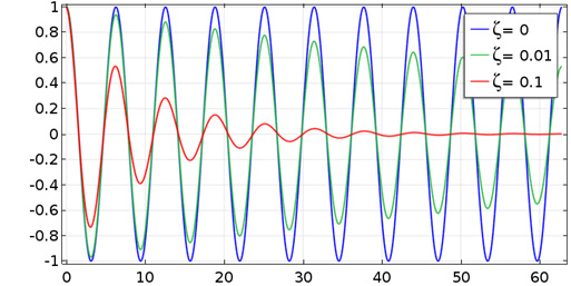
Decay of a free vibration for three different values of the damping ratio.
Another measure in use is the logarithmic decrement, δ. This is the logarithm of the ratio between the amplitudes of two subsequent peaks,
where T is the period.
The relation between the logarithmic decrement and the damping ratio is
Another case in which the effect of damping has a prominent role is when a structure is subjected to a harmonic excitation at a frequency that is close to a natural frequency. Exactly at resonance, the vibration amplitude tends to infinity, unless there is some damping in the system. The actual amplitude at resonance is controlled solely by the amount of damping.
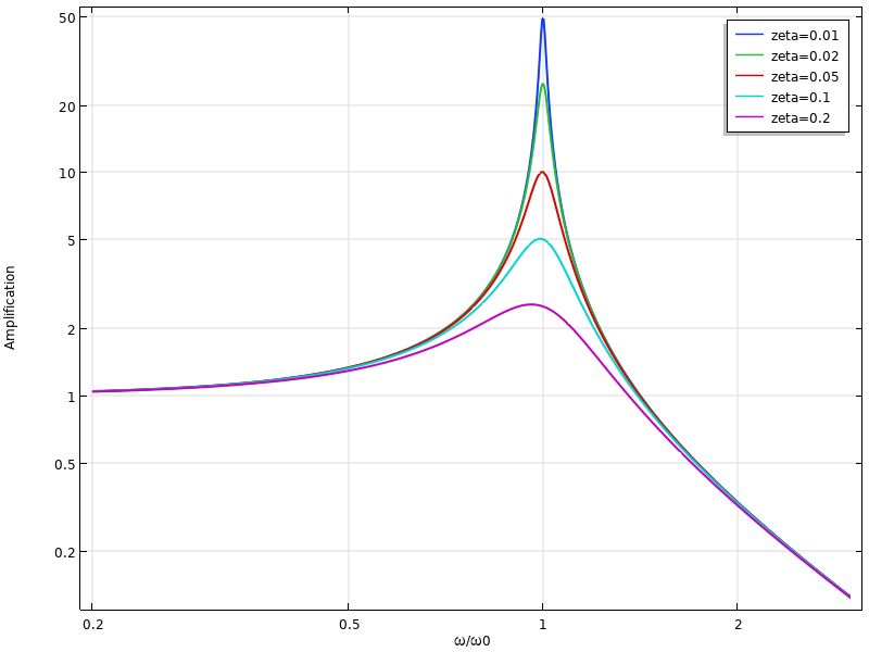
Amplification for a single-DOF system for different frequencies and damping ratios.
In some systems, like resonators, the aim is to get as much amplification as possible. This leads to another popular damping measure: the quality factor or Q factor. It is defined as the amplification at resonance. The Q factor is related to the damping ratio by
Another starting point for the damping description is to assume that there is a certain phase shift between the applied force and resulting displacement, or between stress and strain. Talking about phase shifts is only meaningful for a steady-state harmonic vibration. If you plot the stress vs. strain for a complete period, you will see an ellipse describing a hysteresis loop.
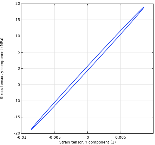
Stress-strain history.
You can think of the material properties as being complex-valued. Thus, for uniaxial linear elasticity, the complex-valued stress-strain relation can be written as
Here, the real part of Young’s modulus is called the storage modulus, and the imaginary part is called the loss modulus. Often, the loss modulus is described by a loss factor, η, so that
Here, E can be identified as the storage modulus E’. You may also encounter another definition, in which E is the ratio between the stress amplitude and strain amplitude, thus
in which case
The distinction is important only for high values of the loss factor.
An equivalent measure for loss factor damping is the loss tangent, defined as
The loss angle δ is the phase shift between stress and strain.
Damping defined by a loss factor behaves somewhat differently from viscous damping. Loss factor damping is proportional to the displacement amplitude, whereas viscous damping is proportional to the velocity. Thus, it is not possible to directly convert one number into the other.
In the figure below, the response of a single-DOF system is compared for the two damping models. It can be seen that viscous damping predicts higher damping than loss factor damping above the resonance and lower damping below it.
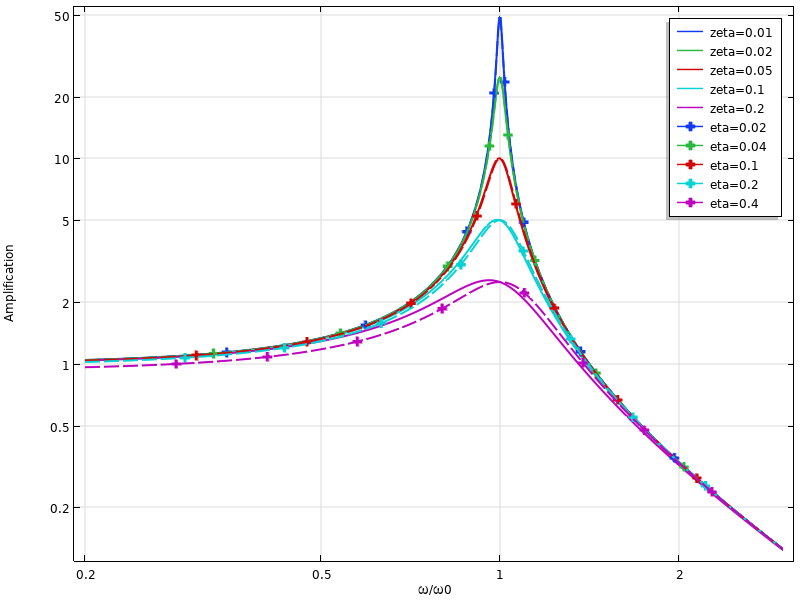
Comparison of dynamic response for viscous damping (solid lines) and loss factor damping (dashed lines).
Usually, the conversion between the damping ratio and loss factor damping is considered at a resonant frequency, and then \eta \approx 2 \zeta. However, this is only true at a single frequency. In the figure below, a two-DOF system is considered. The damping values have been matched at the first resonance, and it is clear that the predictions at the second resonance differ significantly.
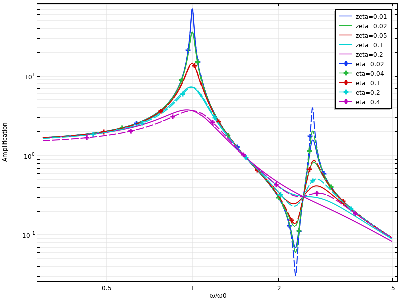
Comparison of dynamic response for viscous damping and loss factor damping for a two-DOF system.
The loss factor concept can be generalized by defining the loss factor in terms of energy. It can be shown that for the material model described above, the energy dissipated during a load cycle is
where \varepsilon_a is the strain amplitude.
Similarly, the maximum elastic energy during the cycle is
The loss factor can thus be written in terms of energy as
This definition in terms of dissipated energy can be used irrespective of whether the hysteresis loop actually is a perfect ellipse or not — as long as the two energy quantities can be determined.
Sources of Damping
From the physical point of view, there are many possible sources of damping. Nature has a tendency to always find a way to dissipate energy.
Internal Losses in the Material
All real materials will dissipate some energy when strained. You can think of it as a kind of internal friction. If you look at a stress-strain curve for a complete load cycle, it will not trace a perfect straight line. Rather, you will see something that is more like a thin ellipse.
Often, loss factor damping is considered a suitable representation for material damping, since experience shows that the energy loss per cycle tends to have rather weak dependencies on frequency and amplitude. However, since the mathematical foundation for loss factor damping is based on complex-valued quantities, the underlying assumption is harmonic vibration. Thus, this damping model can only be used for frequency-domain analyses.
The loss factor for a material can have quite a large variation, depending on its detailed composition and which sources you consult. In the table below, some rough estimates are provided.
| Material | Loss Factor, η |
|---|---|
| Aluminum | 0.0001–0.02 |
| Concrete | 0.02–0.05 |
| Copper | 0.001–0.05 |
| Glass | 0.0001–0.005 |
| Rubber | 0.05–2 |
| Steel | 0.0001–0.01 |
Loss factors and similar damping descriptions are mainly used when the exact physics of the damping in the material is not known or not important. In several material models, such as viscoelasticity, the dissipation is an inherent property of the model.
Friction in Joints
It is common that structures are joined by, for example, bolts or rivets. If the joined surfaces are sliding relative to each other during the vibration, the energy is dissipated through friction. As long as the value of the friction force itself does not change during the cycle, the energy lost per cycle is more or less frequency independent. In this sense, the friction is similar to internal losses in the material.
Bolted joints are common in mechanical engineering. The amount of dissipation that will be experienced in bolted joints can vary quite a lot, depending on the design. If low damping is important, then the bolts should be closely spaced and well-tightened so that macroscopic slip between the joined surfaces is avoided.
Sound Emission
A vibrating surface will displace the surrounding air (or other surrounding medium) so that sound waves are emitted. These sound waves carry away some energy, which results in the energy loss from the point of view of the structure.
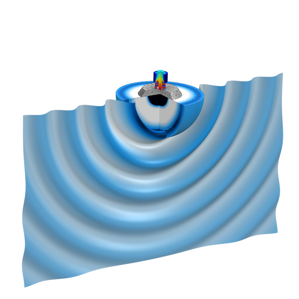
A plot of the sound emission in a Tonpilz transducer.
Anchor Losses
Often, a small component is attached to a larger structure that is not part of the simulation. When the component vibrates, some waves will be induced in the supporting structure and carried away. This phenomenon is often called anchor losses, particularly in the context of MEMS.
Thermoelastic Damping
Even with pure elastic deformation without dissipation, straining a material will change its temperature slightly. Local stretching leads to a temperature decrease, while compression implies a local heating.
Fundamentally, this is a reversible process, so the temperature will return to the original value if the stress is released. Usually, however, there are gradients in the stress field with associated gradients in the temperature distribution. This will cause a heat flux from warmer to cooler regions. When the stress is removed during a later part of the load cycle, the temperature distribution is no longer the same as the one caused by the onloading. Thus, it is not possible to locally return to the original state. This becomes a source of dissipation.
The thermoelastic damping effect is mostly important when working with small length scales and high-frequency vibrations. For MEMS resonators, thermoelastic damping may give a significant decrease of the Q factor.
Dashpots
Sometimes, a structure contains intentional discrete dampers, like the shock absorbers in a wheel suspension.
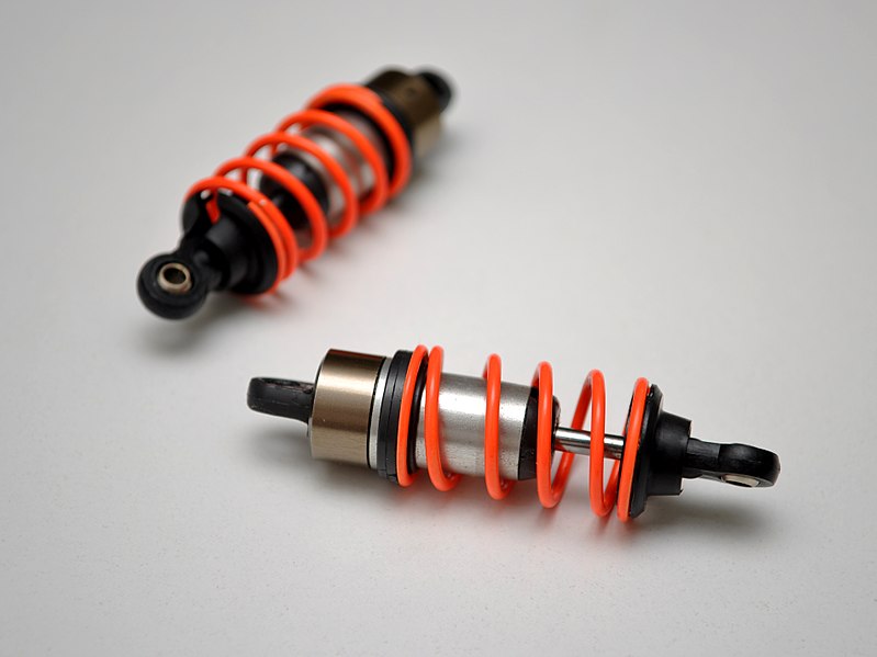
Shock absorbers. Image by Avsar Aras — Own work. Licensed under CC BY-SA 3.0, via Wikimedia Commons.
Such components obviously have a large influence on the total damping in a structure, at least with respect to some vibration modes.
Seismic Dampers
A particular case where much effort is spent on damping is in civil engineering structures in seismically active areas. It is of the utmost importance to reduce the vibration levels in buildings if hit by an earthquake. The purpose of such dampers can be both to isolate a structure from its foundation and to provide dissipation.
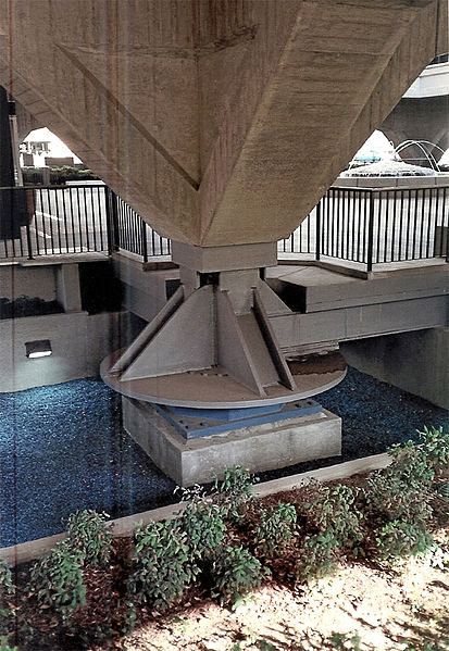
A seismic damper for a municipal building. Image by Shustov — Own work. Licensed under CC BY-SA 3.0, via Wikimedia Commons.
Further Reading
Read the follow-ups to this blog post here:


Comments (16)
Nagi Elabbasi
March 14, 2019Thanks Henrik, this is a very informative blog! Accurately modeling damping I find is a challenge. There is the theory which you describe here, the computational aspects which you will cover I guess in your next blog post, and there is also the experimental determination of the damping constants. That is quite hard in many cases, and may not be even constant across your operating range (may vary with temperature, frequency, and sometimes amplitude of strains/vibrations). Thanks again for an informative blog. Nagi
Stephane Corn
March 18, 2019Dear Henrik,
Thank you for that brilliant recap about structural damping. Very useful.
Stephane
Henrik Sönnerlind
March 18, 2019Thanks for your nice comments!
As for a discussion about the experimental determination of damping parameters, that would be a good topic for a ‘guest’ blog post written by one of our users.
Regards,
Henrik
Ulrik Skov
March 18, 2019Hi Henrik,
Excellent post showing how the resonance peak moves in different directions when damping increase assuming either viscous damping (zeta as function of velocity) or loss factor damping (eta as function of displacement) since the “damping quantity” (zeta or eta) multiplies a different terms in the governing equation for the motion.
Happy sims,
Ulrik
Ivar KJELBERG
March 20, 2019Hi Henrik,
thanks again for an instructive BLOG.
If I read you carefully, a Complex value material properties (complex E, or complex PZT properties) works OK to show damping in frequency domain analysis, periodic oscillations.
But then what about time domain ? How is this handled in COMSOL, since often you do consider complex values, do this provide similar damping for time and frequency domain results ?
Basically I’m at the same point as for my question in the other damping blog 😉
Having fun COMSOLing 🙂
Sincerely
Ivar
Henrik Sönnerlind
March 20, 2019Hi Ivar,
You should not use complex valued inputs in time domain. The complex notation is related to frequency domain, where for example a time derivative is the same as multiplication by i*omega.
The effects of using complex valued input in time domain is unpredictable. In principle you will just solve the same problem as with real input, but at a higher cost because of the complex arithmetic. There are however many potential subtle problems since the variable expressions used in time domain do not expect to operate on complex numbers.
Regards,
Henrik
Abdullah Alshaya
March 20, 2019Hello Henrik,
This is Abdullah Alshaya, I once met you in the COMSOL conference in Lausanne. I have athin plate modeled as 3D in solid mechanics module. On the top of this plate, I have places a mass-spring resonator (vibration absorber) where I have modeled in COMSOL using the lumped mechanical system. I coupled the two systems using the “External Source” from the lumped mechanical system and I exert the reactions from this external source to the solid 3D plate. The eigenfrequencies obtained from the eigenfrequency study matched perfectly the in-house FE code. However, now I am trying to study frequency response to a harmonic force of an amplitude 1 while changing its frequency. Since I am applying the reaction forces from the external source of the lumped mechanical system to the 3D solid plate, how can I apply the harmonic force?
I tried to add to be something like this:
“-lms.E136_f2 + linper(1)”
where “-lms.E136_f2” is the reaction force from the external source and “linper(1)” is my harmonic force but still I could not succeed. I will be really appreciated if I can find an answer from you. I can send you my model.
Thank you
Abdullah
Henrik Sönnerlind
March 21, 2019Hello Abdullah,
Since this is a question about a specific model, please direct it to support (https://www.comsol.com/support), or post your question in the user forum (https://www.comsol.com/forum).
Regards,
Henrik
Abdullah Alshaya
March 21, 2019Hello Henrik,
Thank you very much. I have posted the question in the forum.
Abdullah
René Christensen
April 3, 2019Great post! As Ulrik already stated, I think it is worth noting that the frequency where the response peaks(!) is only equal to the natural frequency, when there is no damping in the system, as can also be seen from the figures.
Henrik Sönnerlind
April 4, 2019Hi Réne,
Based on the comments from you and Ulrik, I will write a separate follow-up blog post discussing frequency response in particular.
Regards,
Henrik
Claudia Borzea
April 6, 2020Awesome blog. I was able to find the damping loss to introduce in COMSOL based on Quality Factor given in my piezoelectric harvester specifications. Beautifully explained. I was very happy to calculate the damping loss rather than wander around trying random values for damping loss in COMSOL. Thank you so much! You made the relations and all very clear.
Xianfeng Chen
August 6, 2020Hi Henrik, thank you very much. Very clear and informative. However, I have a question. In the blog, you say internal loss of material and joint loss are kind of independent from frequency, but you also say loss factor (an index for internal loss of material) can only converted to damping ratio at a certain frequency. If internal loss (loss factor) is independent of frequency, I could convert loss factor to damping ratio at any frequency, right? Could you kindly explain this? Thank you very much.
Babak Haghpanah
July 8, 2021Hi Henrik,
Thanks for the great post!
In one of the graphs you are showing a ‘comparison of dynamic response for viscous damping and loss factor damping for a two-DOF system’. I wonder how zeta (ζ) is defined for this two-DOF?
For a SDOF we have ζ = c / (2*sqrt(k*m)), so with a given ζ value one can calculate the damping coefficient, c.
For the two-DOF, how is ζ in this plot related to m1,2 , k1,2, and c1,2? Is here assumed that c1 = c2 = c, and ζ = c / (2*sqrt(k1*m1))?
Thanks,
Babak
Pietro Ferrari
June 29, 2023Hi Henrik,
thank you for your work.
Could I ask you why there is a range of values for the aluminum loss factor (min: 0.0001 and max: 0.02) ? Does it depend on the particular chemical composition of the aluminum? Maybe a special heat treatment?
Sincerely appreciate your help.
Pietro
Henrik Sönnerlind
June 29, 2023 COMSOL EmployeeThere are probably many different factors, but I am not an expert in that. Some such factors are discussed in this paper: https://www.researchgate.net/publication/229001850_Factors_effecting_internal_damping_in_aluminum