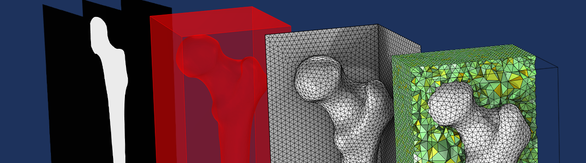
Have you ever wondered how to create a simulation mesh out of data obtained by 3D imaging techniques? In this blog post, we will explain how to do so using the COMSOL Multiphysics® software. This topic expands on the theme of modeling irregular shapes, which we have explored in past blog posts. The processes we will discuss here are, in part, already used when setting up verification studies for topology optimization results. Nevertheless, in this blog post we will generalize the workflow to suit data obtained by 3D imaging techniques.
The Input Data
COMSOL Multiphysics® supports data import on different formats: text files, Excel files, CSV files, images, DEM files, MATLAB® functions, and external functions written in the C programming language. Scanned data often comes in a set of cross-sectional images, including in the example we will look at here: a part of a human femur. Certain data in this model has been obtained from the Visible Human Project. However, COMSOL Multiphysics only supports the import of one image for the generation of 2D data. Therefore, before using the software, the data file was generated by taking the following steps: The images with the upper half of the femurs were handpicked, and the pixels containing one of the femurs were manually identified to reduce the amount of data. The brightness of the identified pixels were, in turn, read and written into a text file along with its position in space. The pixel position in the image represents the x– and y-coordinates, and the image number represents the z-coordinate. The spreadsheet format is a suitable format to use, as each pixel is read from an image and written to a text file one at a time:
x1 y1 z1 data1

x2 y2 z2 data2

x3 y3 z3 data3

...
The data was also cleaned up to remove everything except the femur and was scaled to fit the actual size of the femur. It was also binarized for ease of use.
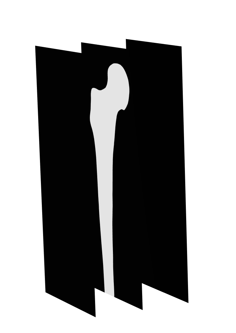
Three slice plots of the binarized data of a human femur that will be used to create a mesh. The white represents the brightness at a value of 1, and the black represents a value of 0 in the data file.
The MPH files can be downloaded at the bottom of this page, so the instructions here will only paint a general picture of the steps you need to take. By the end of this blog post, we will have two meshes of a human femur with a surrounding domain, which we can use for future computations. We will also discuss how to add other computational domains and partition the surface mesh to be able to apply appropriate boundary conditions on the mesh.
To start out, import the data into an Interpolation function in the software. Let’s call the function human_femur. We will go over two possible workflows to arrive at a mesh of the femur:
- A fast track where you get a very crude mesh representation of the data, and where we let the remeshing flatten the rough surfaces
- A workflow containing more steps that use Helmholtz smoothing to make sure we get a smooth shape
Workflow 1: Representing the Data Using a Grid Dataset and Remeshing the Surfaces as a Smoothing Technique
We will start by looking at the faster of the two workflows. In this example, we will represent the data using a Grid dataset and will filter out the data to represent the femur using a Filter dataset. This will generate a surface mesh that is very blocky, so we will use the Free Triangular operation to smoothen the uneven surface.
Setting Up a Grid Dataset and Filtering out the Data of the Femur
For this workflow, we do not need a Geometry node or even a Component node in the Model Builder, though we will add it later when it is time to add extra computational domains and create a computational mesh of the femur. Set up the Interpolation function under the Global Definitions node, and then go directly to Results to define a Grid dataset.
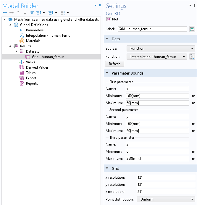
A Grid dataset is set up directly after adding the Interpolation function.
The Grid dataset is used as a regular mesh, and the Interpolation function is applied on this mesh. Here, about half of the image resolution is used for the resolution of the dataset. Now, add a Filter dataset and enter the expression human_femur(x,y,z) and set the Lower bound to
0.99. This will create an isosurface at a value of 0.99, and it will include all data that exceeds that value. In other words, an isosurface for the human femur. The Filter dataset is suitable if you want one domain in the end. In the second workflow, we will instead use the Partition dataset, where you can define several values to create multiple isosurfaces that will result in several computational domains.
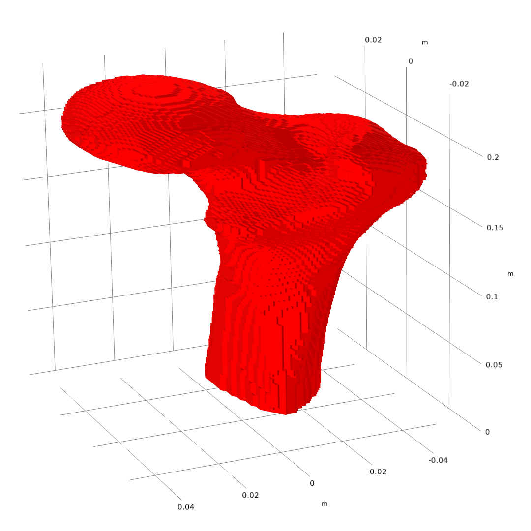
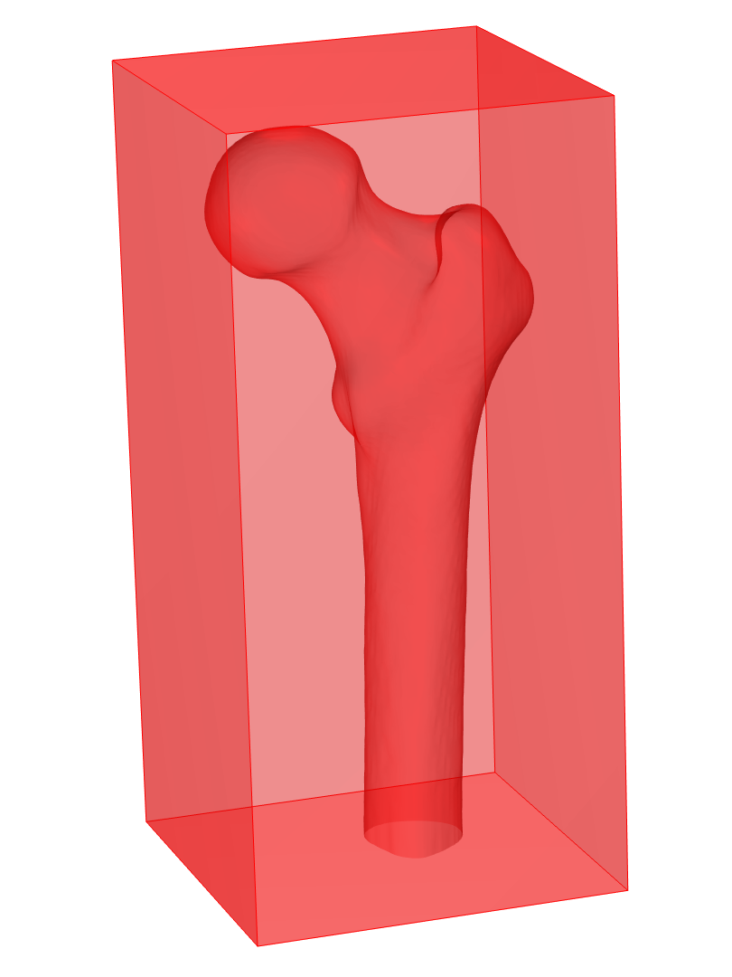
The isosurface generated by the Filter dataset. Note that the femur is compressed in the z direction because the axes are scaled.
Importing and Partitioning the Mesh of the Filter Dataset
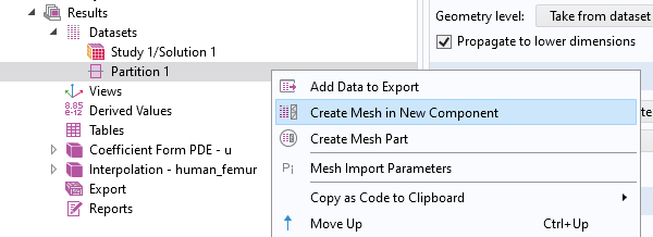
The mesh represented by this Filter dataset can be imported into a meshing sequence where we will remesh the faces to smooth over the roughness. In this workflow, we right-click the Datasets > Filter node and select Create Mesh Part.
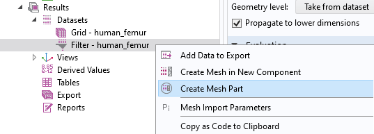
In the second workflow, we will use the Create a Mesh in a New Component option. In this workflow, we choose to create a Mesh Part because we will also use the mesh as construction geometry, which we will see shortly. This automatically sets up a Mesh Part under Global Definitions and adds an Import node that imports the mesh of the Filter dataset. The domain elements of a Filter dataset are often of poor quality, so we will only import the triangle mesh. Then, once we are satisfied with the surface mesh, we will regenerate the tetrahedral mesh.
It’s often common that you need a specific boundary partitioning for applying a boundary condition. Use the Intersect with Plane operation to make planar cuts and the partitioning operations for other shapes. Read the “Editing and Repairing Imported Meshes in COMSOL Multiphysics®” blog post to see a comparison between intersecting and partitioning a mesh. Here, we will use the Partition with Ball operation to get a roughly circular boundary.
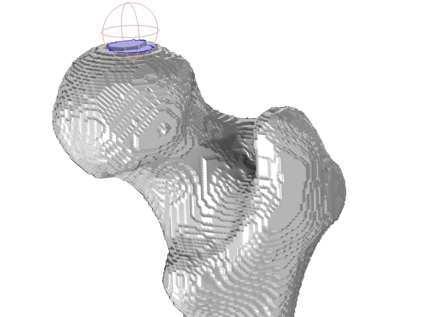
Using the Partition with Ball operation (pink edges) to partition out a roughly circular boundary (highlighted in blue) on which we can later apply a boundary condition. The rendering of the mesh has been turned off for viewing purposes.
Remeshing to Improve Quality and Even Out Roughness
The mixture of element sizes and the many sliver triangles make the mesh unsuitable for simulations. It thus needs to be remeshed before it can be used. Remeshing the faces with a larger mesh size will also smooth out the shape.
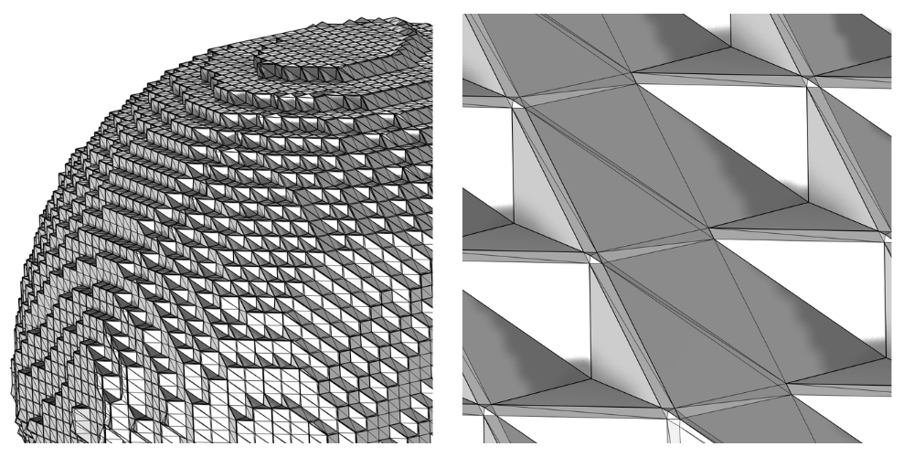
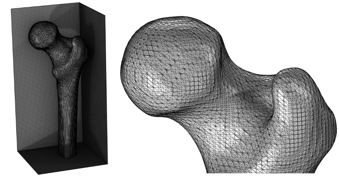
A zoomed-in picture of the imported Filter mesh. This mesh is very blocky in shape due to the hexagonal shape of the grid dataset. It contains a mix of large, small, and sliver triangles.
Use the Remesh Faces operation to remesh the faces. To avoid resolving the roughness in the mesh and instead even it out, set an element size that is larger than the unevenness in the mesh. We can do this by setting both Maximum element size and Minimum element size to 0.005 m. As can be seen in the image below, the surfaces are now smooth enough. However, the boundaries will be remeshed once more at a later stage in the workflow, so the faces will be evened out further.
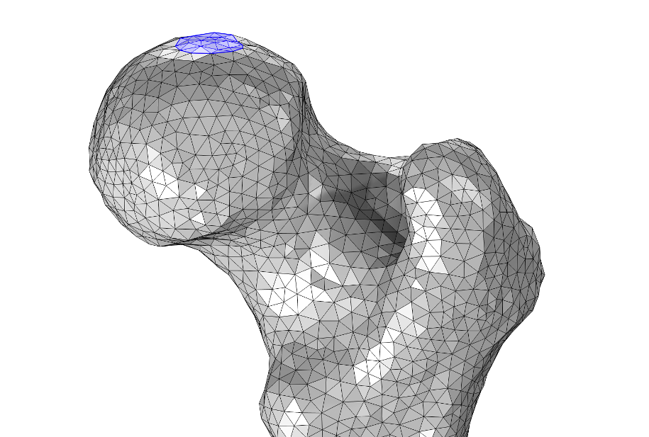
The image shows the top of the femur after remeshing the surfaces once.
If you are trying to remesh surfaces that are almost intersecting one another, or if you are remeshing one surface that is almost intersecting itself, try using Helmholtz smoothing instead.
The surface mesh is now good enough to continue to add extra geometry to this mesh.
Adding More Computational Domains
The domain of the femur might be the only domain you’re interested in, but let’s say that you also want a simulation domain around the femur or some screws to fixate a fracture in the femur. How would you go about doing that? This is accomplished with a Geometry sequence. Start by adding a 3D component to the femur model. Then, add Geometry > Import. In the Settings window of this node, select Mesh Part 1. This node will enable us to add and position new geometry, and should be marked as Construction Geometry since we will only be using the faces of the femur to position said geometry. A construction geometry object is always removed once the geometry is finalized. You can see that it is a construction geometry because the edges are dashed rather than solid.
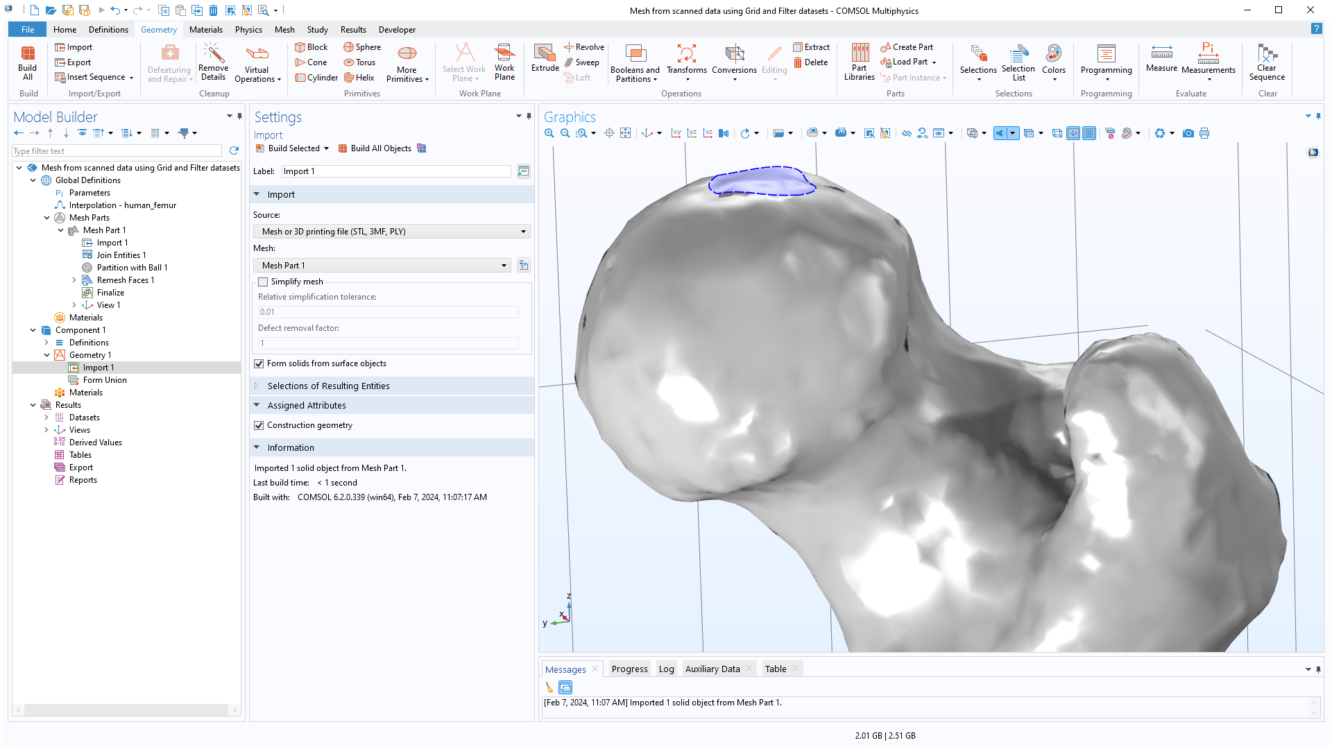
Importing the femur as a Construction geometry object into the geometry sequence to position additional geometry in relation to the femur.
The geometry that we will create will later be combined with the mesh in a meshing sequence. Combining geometry or imported CAD with mesh is usually most robust using the mesh Union operation in a mesh sequence, and this is the workflow we will follow here.
You can draw any geometry you need for your simulations or import a CAD design. With the construction geometry available, it is easy to draw the desired geometry. In this example, we will add two screws to reinforce the femur, but the principle is similar regardless if you create or import one or several geometry objects. The geometry of the screws together with the construction geometry of the femur is seen in the left image below. Once the geometry is complete and you have built the Form Union, the construction geometry of the femur is removed from the resulting geometry, which leaves only the screws, as seen in the middle image below. For imported CAD designs, you can also add Remove Details nodes or Virtual operations to simplify your geometry before combining it with the mesh. For more detailed instructions on how to combine geometry and mesh, see the second tutorial in the STL Import Tutorial Series.
In the same Component, go over to the Mesh sequence. Make sure to add two Import nodes, one importing the geometry of the screws, and one Import node importing the mesh of the femur from the mesh part (right image below). Unite the two surface meshes with a mesh Union operation, then join the domains of the screws with Join Entities, as they were partitioned in two by the face of the femur.
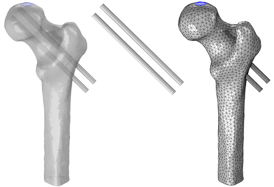
Left: The geometry of the screws with the construction geometry of the femur. Middle: The geometry of the screws after building the Form Union node. Right: The mesh of the femur and the screws imported into a meshing sequence.
Remesh the faces of the femur using a Remesh Faces node with Maximum element size and Minimum element size set to 0.005 m. Make sure to add a Fixed Mesh attribute to the Remesh Faces operation and select to keep the mesh on the edges of the screw holes fixed (highlighted in blue image at left below). This improves the element quality of the mesh around the screw holes and also smoothens the face of the femur further.
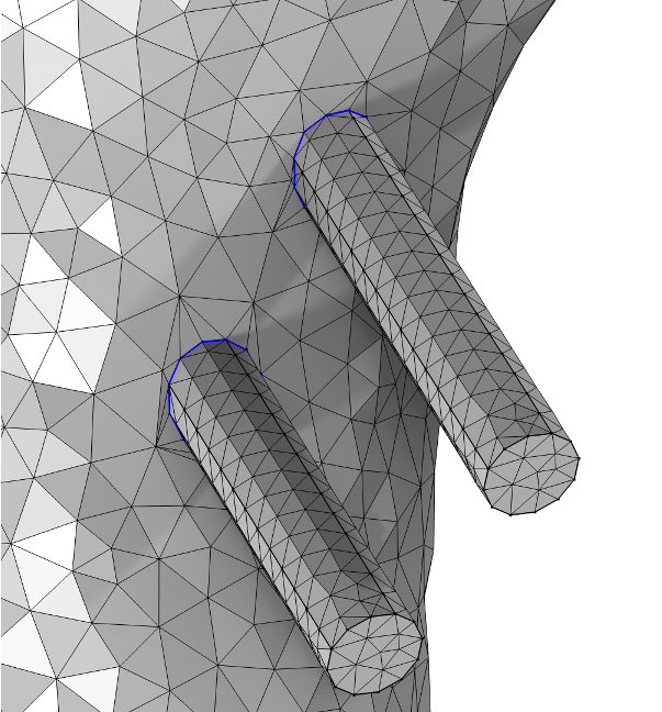
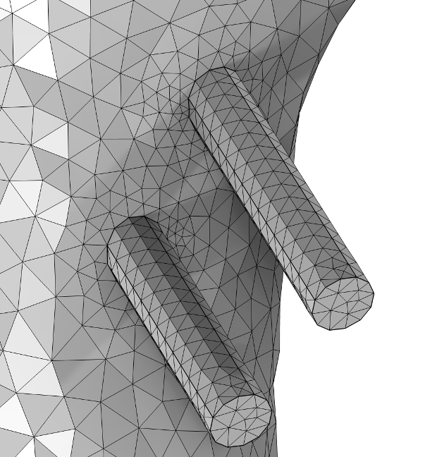
Remeshing the faces of the femur a second time while keeping the edges around the screw holes fixed.
Lastly, add a Free Tetrahedral operation to fill the domains with a tetrahedral mesh. There is an option to add a swept mesh or boundary layer mesh, if that is needed for the physics at hand. The domains and boundaries defined by this mesh will be used when you set up and solve your simulations.
Adding Physics with Higher-Order Discretization
The mesh is now ready for simulations, seen in the left image below. But what happens if we add physics with higher-order discretization? Let’s say that we want to set up a solid mechanics simulation, which uses the discretization setting Quadratic serendipity. The second-order nodes of the curved elements will then be placed on a curved representation of the mesh surfaces, similar to how they are placed when you have an underlying geometry. To get an idea of what the curved elements look like in our mesh, we can set up a Mesh plot by setting Geometry shape function to Quadratic Lagrange for the mesh dataset and Node points to Geometric shape function for the plot. The Quadratic Lagrange plot setting is not coupled with any physics discretization in the model; it is only used for plotting.
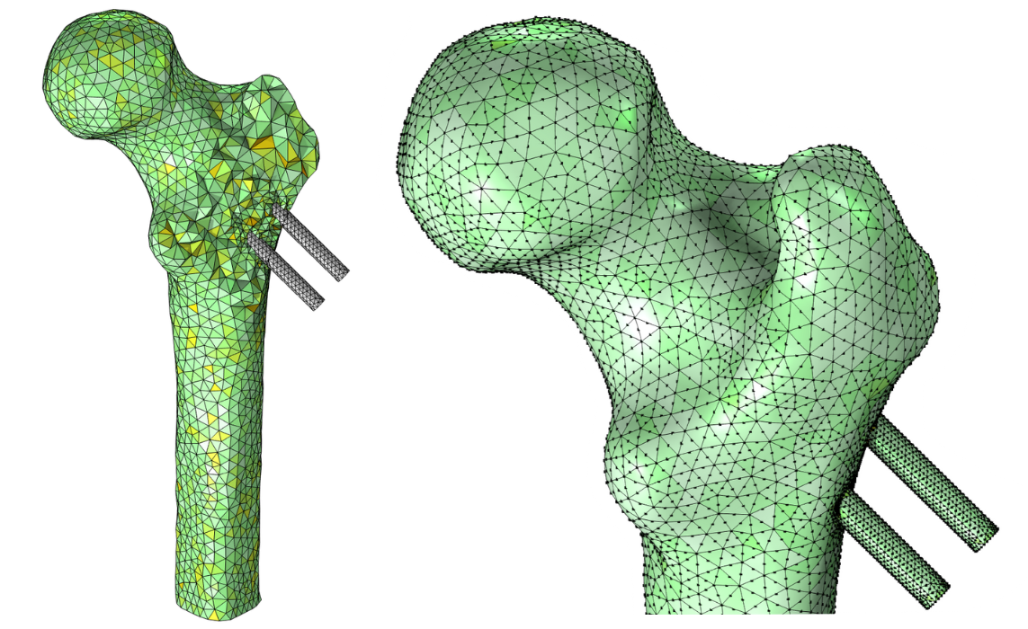
Left: A mesh plot of the volume mesh of the femur and screws. The white elements represent the domains of the screws, and the elements of the femur are filtered by the expression x > -0.015. Right: The final mesh with the second-order node points displayed on the curved boundary of the femur. The green and yellow represent the skewness.
Comparison of Generated Mesh and Imported Data
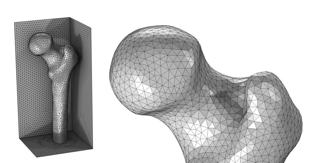
As a way of comparing how the generated mesh follows the data, we can add an Isosurface plot of the expression human_femur(x,y,z), plotted on the mesh resolution of the Grid dataset. The mesh follows the isosurface quite well, as can be seen in the image below.
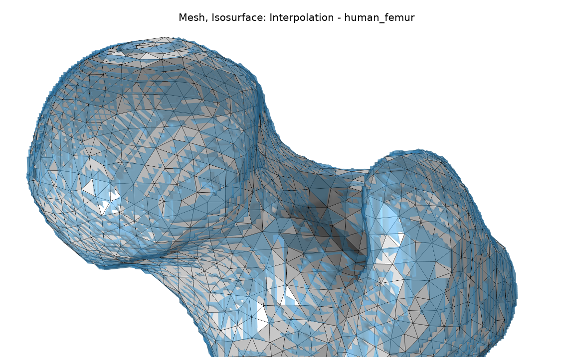
Comparison of the generated surface mesh (gray) and an isosurface of the interpolation data human_femur(x,y,z) (blue).
Workflow 2: Smoothing the Data of the Femur Using Helmholtz Equation
For this workflow, in short, we will add a regular block domain on which the femur data is applied. We solve the Helmholtz equation to smoothen the data, which gives us a smooth surface mesh of the femur. We will still need to remesh the surface mesh of the femur, but this time it will only be to improve the quality of the mesh elements.
Define a Regular Domain
In order to solve Helmholtz equation, you need a domain. This domain can be a block, sphere, or some other simple shape in which the data of the femur will fit, as discussed in this blog post. You want to keep this domain as small as possible so that you can resolve the domain with a fine mesh. The mesh needs to be fine enough to resolve any details in the data that you want to see in the surface mesh.
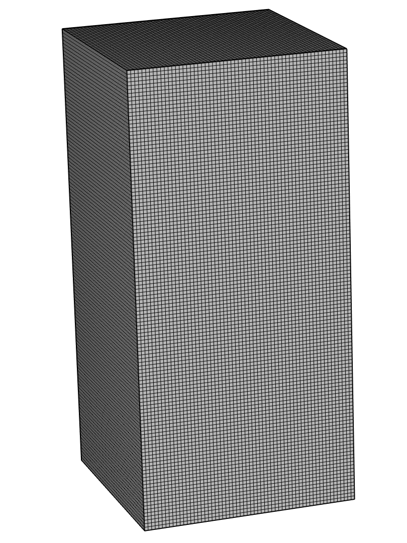
A fine-enough hexahedral mesh on a regular domain where the imported data is defined.
Next, set up the equations, add a stationary study, and solve it to gain access to a solution dataset that we can use.
Helmholtz Smoothing of the Data
To avoid numerical artifacts and make it possible to use a slightly coarser mesh, the interpolation function is low-pass filtered using a Helmholtz-filtered PDE:
where R is the filter radius representing approximately the width of the low-pass filter. Add a Coefficient Form PDE interface, as shown in the image below.
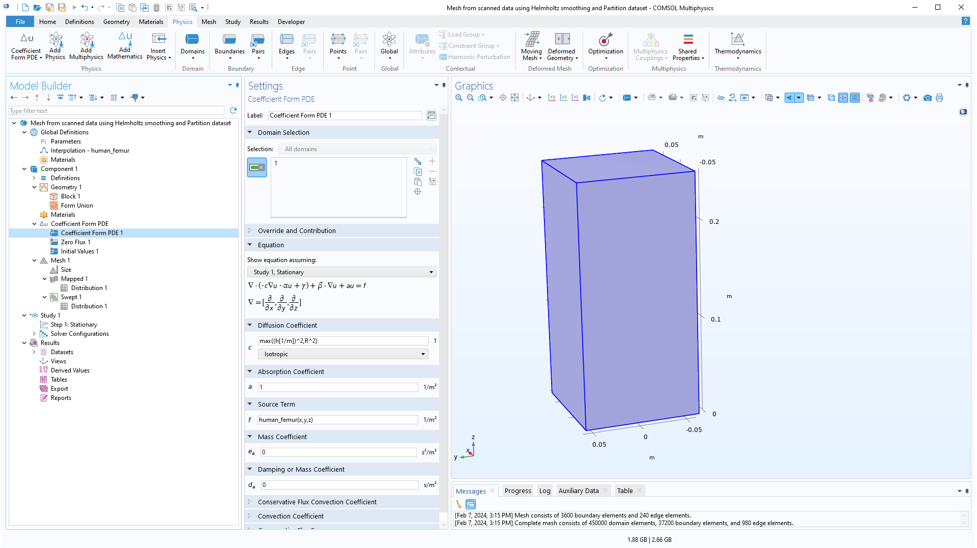
Settings for the Coefficient Form PDE interface.
Here, we use the expression max((h[1/m])^2,R^2) for the diffusion coefficient. The software will use the largest of the mesh sizes, h, and the parameter R for each node in the mesh. In this example, the local mesh size, h, is constant, but if you use an unstructured tetrahedral mesh, h will vary. Note that since all operations are performed on a geometry represented by a mesh where each element is linear, all element discretization orders are lowered to linear elements. A stationary solver is used to compute the solution.
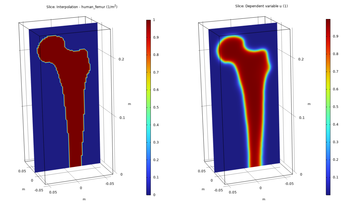
Slice plots of the interpolation function human_femur plotted on the hexahedral mesh (left) and the smoothened solution data (right).
Filtering Out the Femur Using a Partition Dataset
We use a value between 0 (blue) and 1 (red) in the smoothened solution data to filter out a surface mesh of the femur. In this example, assume that we also want the region outside the femur to be part of our simulation. Therefore, we should select to add a Partition dataset. If you are only interested in the domain of the femur, use a Filter dataset instead, as done in the first workflow. For a Levels value of 0.6, the Partition dataset is good enough for our purposes, as seen in the image below.
Plot of the Partition dataset with Levels set to 0.6. The isosurfaces partition the simulation domain into one domain for the femur and one for the surroundings.
When you are satisfied with the levels, right-click the Partition or Filter dataset node and select Create Mesh in New Component. If you need to create additional simulation domains, use the Create Mesh Part option and follow the steps in the first workflow.
This automatically sets up a new component with an Import node to import the mesh of the Partition dataset. Keep the Import domain elements check box cleared and set the Boundary partitioning setting to Minimal. This will import the surface mesh only, and will form as few boundaries as possible; seven planar boundaries and one boundary for the femur. We will improve this surface mesh and then recreate a volume mesh.
Imported Partition dataset mesh. The surface mesh of the femur contains a mixture of large, small, and sliver triangles and its quality needs to be improved to be suitable for simulations. Some boundaries are hidden for viewing purposes.
Remeshing the Surfaces to Improve the Quality of the Triangles
The surfaces are remeshed in the same meshing sequence using the Remesh Faces operation. To get triangles of similar size, the Maximum element size and Minimum element size have both been set to 0.005 m.
The remeshed faces of the femur and block. The size has been modified to generate a surface mesh with similar sized triangles. Some boundaries are hidden for viewing purposes.
The domains can now be filled with a tetrahedral mesh. The physics interfaces that you add will be applied on the domains and boundaries defined by this mesh. We now have a good-quality volume mesh that is ready for simulations. For other shapes and applications where it is needed, it is possible to add a swept and boundary layer mesh to the domains, but in this case we are satisfied with a tetrahedral mesh.
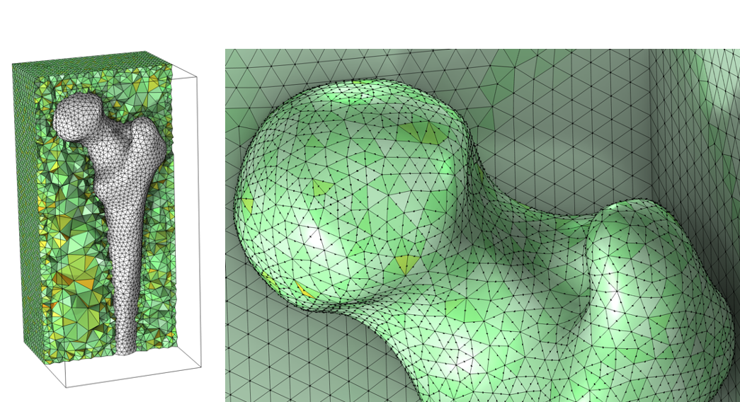
Left: The volume mesh of the femur and surrounding block. The white elements represent the domain of the femur, and the surrounding elements are filtered by the expression x > 0. Right: The final mesh with the second-order node points displayed on the curved boundary of the femur. The colors represent the skewness. Some boundaries are hidden for viewing purposes.
Comparison of Generated Mesh with the Imported and Smoothened Data
The mesh generated in this workflow can be compared with an isosurface, human_femur(x,y,z), of the imported data at the same level as was used for the Partition dataset. This isosurface is plotted on the mesh in the original block domain. To generate a mesh that follows the imported data even closer, use a finer mesh in the original block domain on which the Helmholtz equation is solved. With a smaller mesh size, you can also decrease the diffusion coefficient.
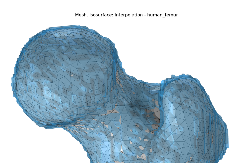
Comparison of the generated surface mesh (gray) and an isosurface of the interpolation data human_femur(x,y,z) (blue).
Concluding Thoughts
With this, we conclude our blog post on creating a surface mesh from scanned data. We have partitioned the surface mesh, smoothened out the data using two different techniques, and have learned how to combine mesh and geometry.
To find more details on the workflows discussed here, download the MPH files via the button below.
Further Resources
- Learn more about meshing in our “Editing and Repairing Imported Meshes in COMSOL Multiphysics” blog post
- Learn more about editing and remeshing imported meshes, as well as combining it with geometry, in the STL Import Tutorial Series
- See another example of data that can be used to create a surface in our “How to Build Geometries from Elevation Data to Model Irregular Shapes” blog post
- Discover three ways to inspect a mesh in our “How to Inspect Your Mesh in COMSOL Multiphysics®” blog post
Editor’s note: This blog post was updated on 4/19/2024 to reflect new features and functionality in COMSOL Multiphysics® version 6.2.
Certain data in this model has been obtained from the Visible Human Project, https://www.nlm.nih.gov/research/visible/visible_human.html, Courtesy of the U.S. National Library of Medicine. Such data is current as of April 21, 2023, and has been modified and may not reflect the most current/accurate data available from NLM. NLM has not endorsed COMSOL’s products, services, or applications and disclaims all warranties, express or implied, including any warranty of merchantability or fitness for a particular purpose, regarding the accuracy or completeness of the data. Users of the data shall hold NLM and the U.S. government harmless from any liability resulting from errors in the data. NLM disclaims any liability for any consequences due to use, misuse, or interpretation of information contained or not contained in the data.
MATLAB is a registered trademark of The MathWorks, Inc.


Comments (2)
Said Bouta
April 26, 2023Thank you for your explanation of generating a simulated Mesh of a Femur From 3D Data.
If I have sequential binary images (black and white), how can I export these images in Comsol to get a 3D model, knowing that these images are obtained with 3D Blender software.
Bests.
Hanna Gothäll
May 2, 2023 COMSOL EmployeeDear Said,
Thank you for your comment. Please click the pink “Try the tutorial model” button above to download all files relating to this blog post. Your images need to be converted into a similar text file before you start working in COMSOL Multiphysics. After that is done, you can follow the steps in the blog post along with the setup of the two example MPH files. If you need further help, please send your questions along with all related files (text file, MPH file, and possibly the image files) to our support: https://www.comsol.com/support/case or support@comsol.com.