
Did you know that you can use the Study node to perform programmatic sequences of operations, including solving the model, saving it to file, and generating and exporting plot groups, results, and images? In this blog post, we take a closer look at this useful capability.
Editor’s note: The original version of this post was published on June 21, 2017. It has since been updated with new content and screenshots.
Example: Micromixer Model
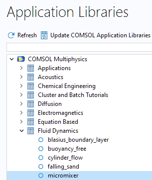
To demonstrate this functionality, we will load the Micromixer tutorial model from the Application Libraries. This model is available in the folder COMSOL Multiphysics > Fluid Dynamics and illustrates fluid flow and mass transport in a laminar static mixer.
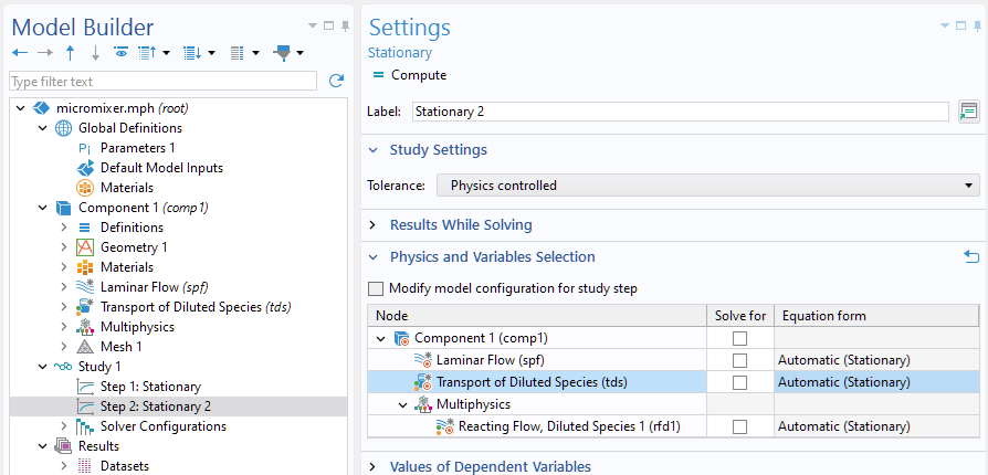
The model first performs a fluid flow simulation using the Laminar Flow interface. In the next step, it calculates the mixing efficiency by means of a Transport of Diluted Species interface, using the results from the fluid flow simulation as input. The species is transported downstream based on the fluid velocity.
The computation time for this model is a few minutes. To simplify the model a bit so that we can run the computation quicker, we won’t solve for the species transport. To achieve this, we will modify the settings of the second study step, Step 2: Stationary 2, by clearing the Transport of Diluted Species and Reacting Flow, Diluted Species checkboxes in the Settings window.
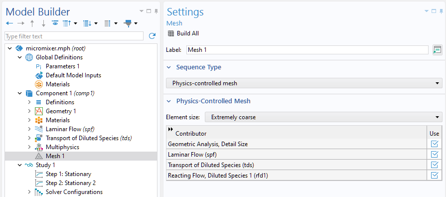
We can make an additional change to run the model faster. In the Mesh node settings, we will set the Sequence type to Physics-controlled mesh and the Element size to Extremely coarse.
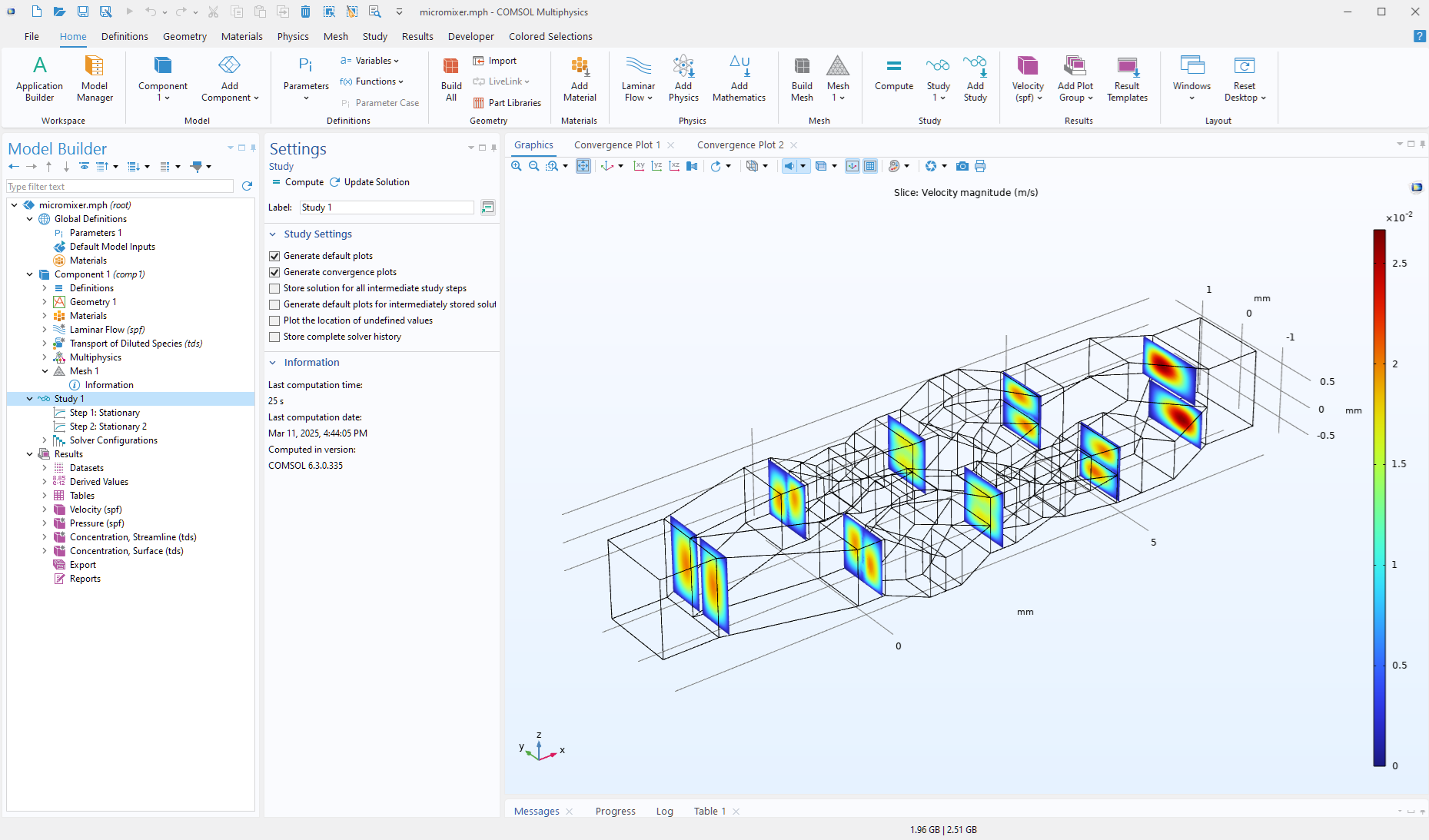
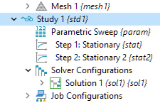
Now, we can compute Study 1 to make sure everything works. The resulting plot shows the velocity magnitude at a few slices along the mixer geometry.
Using Job Sequences to Save Models Automatically
Now that we have prepared the model, we can use a job sequence to automate the process of solving and saving it.
To define a sequence of operations under the Study node, first open the Show More Options dialog by clicking the corresponding button (the “eye” icon) in the Model Builder toolbar. Then, select the Solver and Job Configurations checkbox.
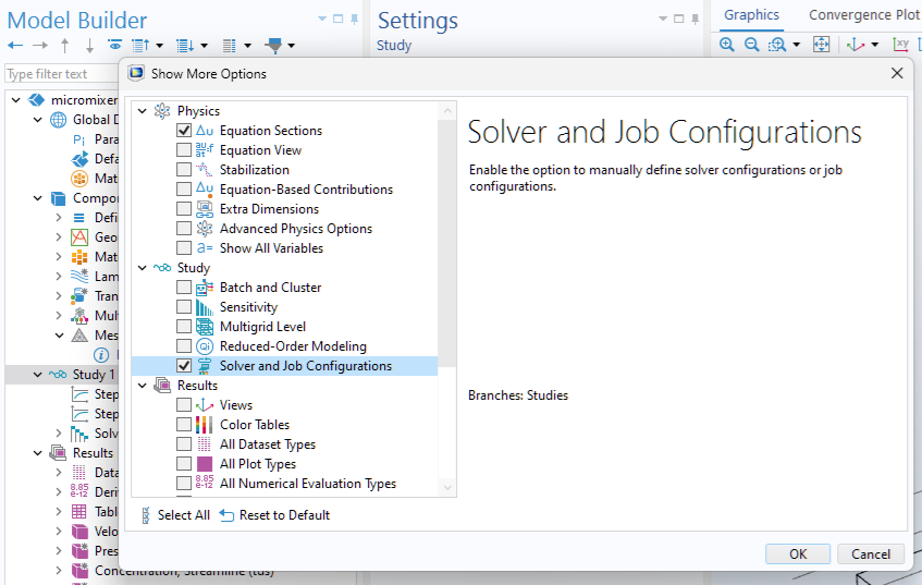
Enabling this setting reveals a hidden Job Configurations node in the model tree. This node is something that you don’t need to worry about during conventional modeling work. It essentially stores low-level information pertaining to the order in which the solution process should be run. Normally, this ordering is controlled indirectly from the top level of a study without the need to enable the Solver and Job Configurations option.
Right-click Job Configurations and select the Sequence option to add a Sequence subnode.
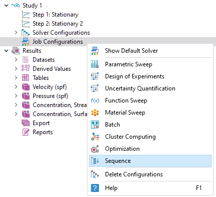
Next, right-click the Sequence node to view, below the Run option, a variety of options that can be added as sequential operations when running the sequence.
- Job — You can use the Job option to add another job configuration to be run from this sequence.
- Solution — The Solution option runs one of the Solution nodes found under the Solver Configurations node further up in the Study tree.
- Other — Under Other, you can select External Class to call an external Java class file. The Geometry option builds a Geometry node, which can be useful, for example, when combined with a parametric sweep to generate a sequence of MPH files with different geometry parameters. The Mesh option builds a Mesh node. The Method Call option calls a method that was added under Global Definitions and created in the Application Builder.
- Save Model to File — Save Model to File saves the solved model to an MPH file.
- Results — Under the Results option, you can choose Plot Group to run all or a selected set of plot groups. Using the Plot Group options automates the generation of plot groups, which means you don’t have to manually click through all of the plot groups after solving to generate the corresponding visualizations. The Derived Value option is there for legacy reasons, and we recommend that you use the Evaluate Derived Values option, which will evaluate nodes under Results > Derived Values. The option Export to File runs any node for data export under the Export node.
Note: All operations performed by adding a Sequence node can also be achieved by writing API code in Java and using the Method Editor. In general, any operation performed in the user interface can also be executed through the COMSOL API.
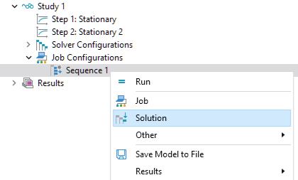
Let’s now create a simple sequence. Right-click the Sequence node and select the Solution option.
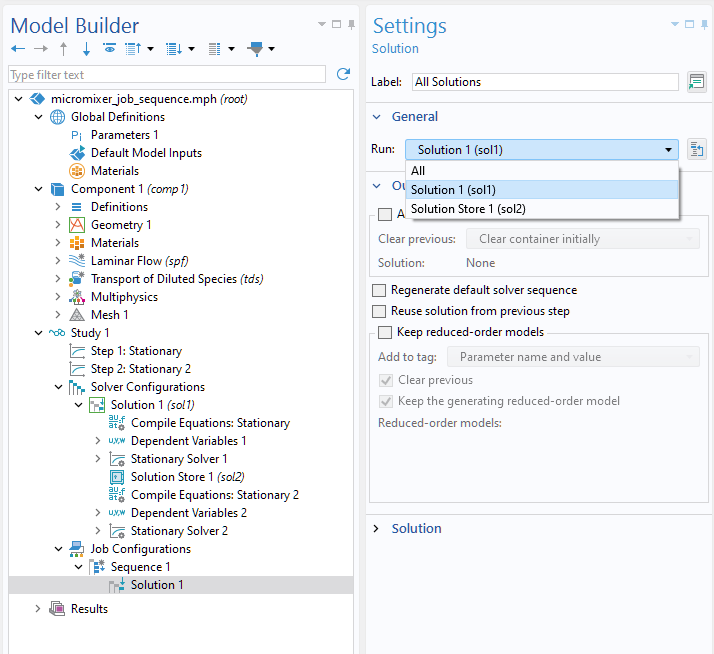
In general, depending on the model and its studies, multiple solver sequences will be defined by different studies. In the General section of the Solution node’s settings, the Run setting allows you to specify which solver sequence(s) to compute. By default, the All option runs all solver sequences under Solver Configurations for all studies. Typically, you will want to set the Run setting to the specific solver sequence you intend to run.
In this example, the solver sequence Solution 1 (sol1) consists of the operations listed under Solver Configurations > Solution 1. Meanwhile, the solution data structure Solution Store 1 (sol2) serves as auxiliary storage for the solution computed by Stationary Solver 1 and is not associated with a solver sequence. Therefore, in this case, we will select Solution 1 (sol1).
When the solver has finished, we’ll want to save the file. To do so, right-click the Sequence node and select Save Model to File.
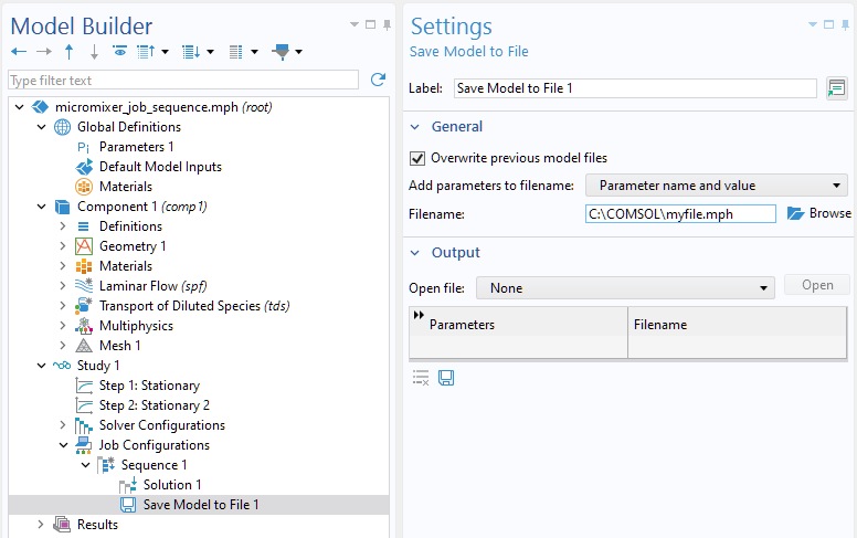
In the Save Model to File settings window, you can see a number of options for saving a series of MPH files with parameters added at the end of the filename. These options are useful for parametric sweeps such as batch sweeps. However, we will not need to do this in such a simple example, so we will select the None option for the Add parameters to filename setting. At this stage, we also need to give a filename to a location where we have permission to write. In this example, the filename and file path is C:\COMSOL\myfile.mph.
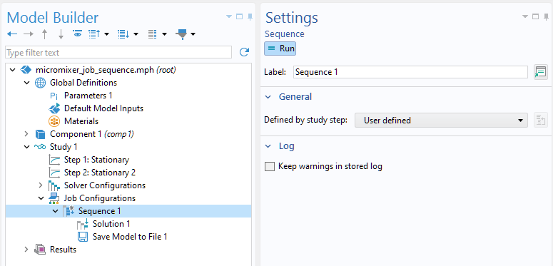
To run these operations, select the Sequence node and click Run.
Exporting Data After Solving in COMSOL Multiphysics®
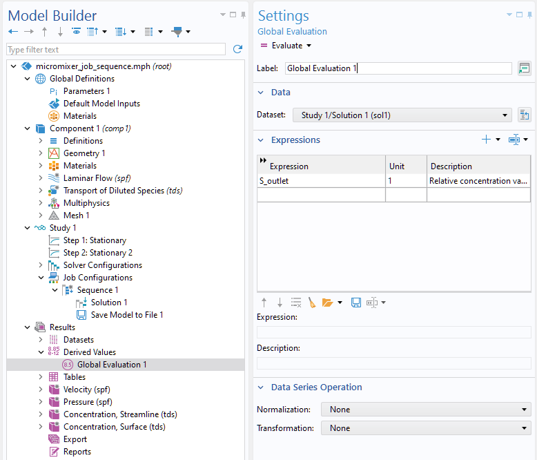
The Micromixer library model we have been using already has one defined derived value. You can see this under Results > Derived Values > Global Evaluation. The variable is called S_outlet and is the relative concentration variance at the outlet. It is defined as a variable under Component > Definitions > Variables.
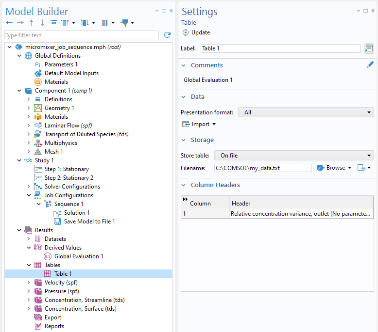
The value of S_outlet is sent to Table 1. We can store this value on file by changing a setting in the Settings window of Table 1. Change Store table to On file and type a filename, e.g., C:\COMSOL\my_data.txt.
Now, add an Evaluate Derived Values operation to the sequence.
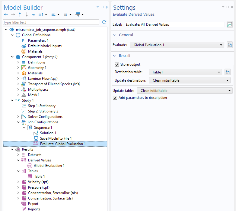
In the General section of the Evaluate Derived Values node settings, if you wanted to evaluate all quantities, you could change the Evaluate setting from All to Global Evaluation 1. Note that selecting this option changes the name of the node in the model tree to Evaluate: Global Evaluation 1. However, in this simple example model, with just one model tree node to evaluate, you can omit this step.
In the Result section, change the Destination table to New
The last step before running the sequence again is to enable the Transport of Diluted Species interface and the Reacting Flow, Diluted Species option in the Settings window of Step 2: Stationary 2 to solve for the species transport (which we initially skipped to run the model faster).
Now, we can run the sequence.
Running Job Sequences from the Study Level or the Command Line
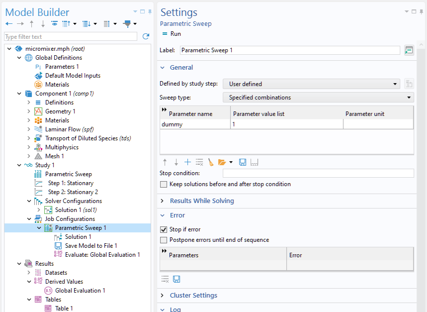
To run a job sequence from the main Study node or the command line, you can use a Parametric Sweep instead of the method described above. A Parametric Sweep is a special type of job sequence, and essentially the same instructions as above apply. However, in this case, the Job Configurations > Parametric Sweep node fills the role of the Job Configurations > Sequence node.
Before adding the Parametric Sweep node, delete the Job Configurations > Sequence node and its child nodes.
Then, add a Parametric Sweep under Study 1. However, by default, the top-level Study node does not recognize job sequences under Job Configurations. Similarly, the command-line interface does not allow direct execution of job sequences within a Study node; it only supports running entire studies. Adding a dummy parameter (e.g., dummy = 1) under Global Definitions > Parameters introduces the necessary overhead for recognition, enabling execution directly from Study 1 as well as via the command line.
This is how the corresponding Parametric Sweep will appear:
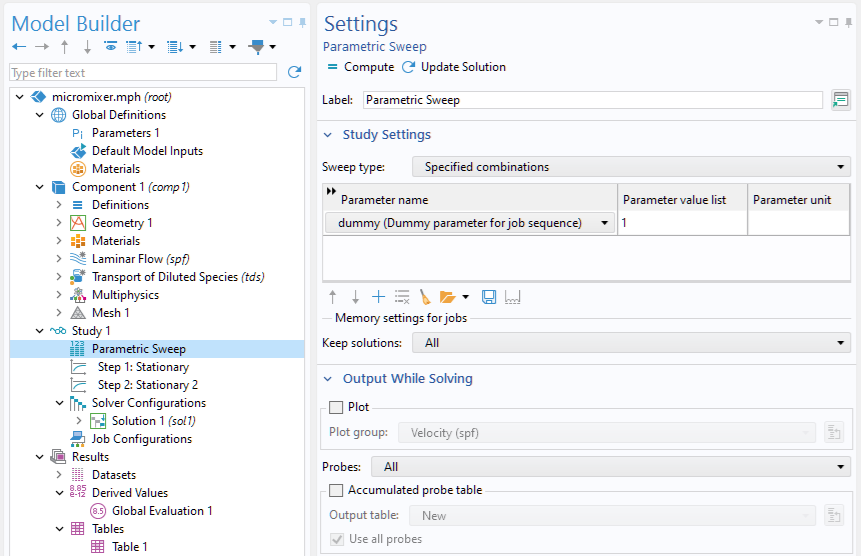
Now, right-click Study 1 and select Show Default Solver. This will add a Parametric Sweep node under Job Configurations.
Note: If you are using a different model, you may first need to switch Use parametric solver: to Off in the Advanced Settings of Study 1 for the
node to appear under Job Configurations.
The following figure shows the corresponding sweep over one parameter value for a dummy parameter. Now, knowing that the Parametric Sweep 1 node is just a special type of Sequence node, we can add Save Model to File and Evaluate: Global Evaluation nodes to go with the automatically created Solution child node. These child nodes operate just as they did in the previous example using a Sequence node.
To run the job sequence from the Model Builder, right-click the Study 1 node and select Compute.
Using the Command-Line Interface
If you are using the command-line interface (e.g., the Command Prompt window in the Windows® operating system) to run the job sequence, once you have added the dummy parameter, you can type a command such as:
comsolbatch -inputfile mymodel.mph -study std1,
where std1 is the tag for Study 1, and mymodel.mph would be replaced with the real filename.
To run this command in the Command Prompt, we need to complete the following steps:
- Confirm the path to the COMSOL® executables has been added to the PATH environmental variable.
- Open the Command Prompt and navigate to the directory containing your input file.
- Enter the command and hit Enter to run it.
See the blog How to Run COMSOL Multiphysics® from the Command Line for more information on using the command line.
In this example, we have added the path to the COMSOL® executables to the PATH environmental variable and changed the directory to the location of the input file before running the command.
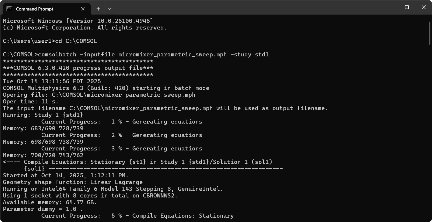 The Command Prompt window where the directory has first been changed to the location of the input file before running the example command.
You can see the progress of the command as it runs. When it is complete, information such as the save location and total time will be displayed.
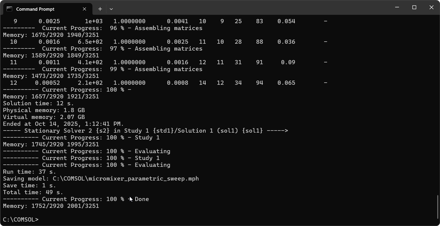 Results of a completed command are shown at the bottom of the Command Prompt window.
If path to the COMSOL® executables has not been added to the PATH environmental variable, the location of comsolbatch.exe needs to be specified in the command. If we set the directory to the location of the input file, in this case C:\COMSOL, and we use the default path to comsolbatch.exe, the version the command would be as follows:
C:\Program Files\COMSOL\COMSOL63\Multiphysics\bin\win64\comsolbatch -inputfile micromixer_parametric_sweep.mph -study std1
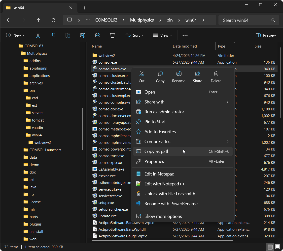 The path to the comsolbatch.exe file is copied from the File Explorer.
Just like when running the study from the COMSOL Desktop®, this command executes the sequence of operations that solves, saves the model to file, and finally evaluates the Global Evaluation node. Note that if you only have one Study node in your model, you can skip the input argument study std1.
To display model tree tags, select Tag from the Model Tree Node Text menu, available in the Model Builder toolbar.
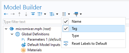
The study tag std1 is now visible in the model tree:
Note that if you already have a parametric sweep in your model, each sweep will be either an “inner sweep” or “outer sweep”. The sweep in the example above using the dummy parameter is an “outer sweep”. The Study node will autodetect which type of sweep to use for best performance, but you can determine this manually if needed. In order to use a job sequence from the command line, your sweep needs to be an “outer sweep”.
More or less all types of sweeps can be changed from being an inner sweep to an outer sweep, but not the other way around. Inner sweeps can be faster, since they will use some of the underlying structure of the computation to speed things up. However, not all types of sweeps can be inner sweeps. For example, a sweep over a geometry parameter always needs to be an outer sweep; again, this is handled automatically by the solver. To make sure the parameter sweep is an outer sweep, change the Use parametric solver to Off in the Parametric Sweep settings; then, perform a Show default solver operation and continue from there.
Next Steps
Job sequences can be used to automate a number of common tasks after solving a model. In this blog post, we demonstrated how to:
- Save the model to file as an MPH file
- Export Derived Values to file
There are other tasks that use job sequences that you can try on your own, including:
- Regenerating all plots after solving
- Exporting plot data to file
- Exporting image data to file
We hope you find that job sequences are a useful feature for your everyday modeling work!
Oracle and Java are registered trademarks of Oracle and/or its affiliates. Microsoft and Windows are either registered trademarks or trademarks of Microsoft Corporation in the United States and/or other countries.


Comments (4)
Daniele Stefanini
June 23, 2017Good morning,
very good post, exactly what I was looking for and even more simple than using an App or writing Java code….thank you !
With this method I can run simulations over night and find the job fully completed the day after
Daniele
Bjorn Sjodin
June 23, 2017 COMSOL EmployeeHi Daniele,
Good to hear that you found it useful.
Best regards,
Bjorn
Daniele Stefanini
August 23, 2017I have a question.
I have multiple files, which I want to launch by using a comsolbatch .bat file.
For each file, I would like to perform the Sequence (there is only one…) included within “Job Configuration”
The Sequence is doing following things :
– solve the problem
– store the file
– plot all
– export all
Is there any argument I can use in the comsolbatch to perform this operation ?
Thanks,
Daniele
Bjorn Sjodin
August 23, 2017 COMSOL EmployeeHi Daniele,
This can be done by first enabling Advanced Study Options and then adding a Batch job node under Job Configurations. The Batch job node is very similar to a Sequence so you can then add your desired sequence of commands under Batch instead of under Sequence. Then call the comsolbatch command with the additional argument -job b1
where b1 is the “tag” of the Batch sequence. You can see this tag displayed in the Properties window (to see it, right-click and select Properties).
The details of how you would do this depend on the exact nature of what you are trying to achieve. I suggest that you contact our support team for further assistance since the details can become quite specific to your model.
Best regards,
Bjorn