From tiny cellphone chargers to large-scale generators, transformers are used to increase, decrease, and isolate voltages in all sorts of applications. While these electrical devices have a pretty simple structure, optimizing their performance can be challenging, as it involves accounting for the coupling of magnetic and electric fields, the behavior of ferromagnetic materials, and more. To analyze these effects, engineers designing transformers can use the COMSOL® software.
Transformers: Increasing, Decreasing, and Isolating Voltage
There are three main types of transformers, and each offers different capabilities:
- Step-up transformers increase voltages
- Step-down transformers decrease voltages
- Unity transformers isolate voltages
Due to these abilities, each type of transformer has a wide range of applications. Large step-up transformers, for example, increase the voltage generated by power plants so that it can be sent over long distances, while smaller versions are often found in microwave ovens and uninterruptible power supply systems. Step-down transformers are used for cellphone chargers, welding, and televisions. Meanwhile, unity transformers are important for meeting safety regulations and are even a legal requirement for certain medical diagnostic equipment. Unity transformers are also used to test electronic devices, supply power to devices high above the ground (such as air traffic warning lamps on radio antenna masts), and mitigate galvanic corrosion in underwater marine applications.
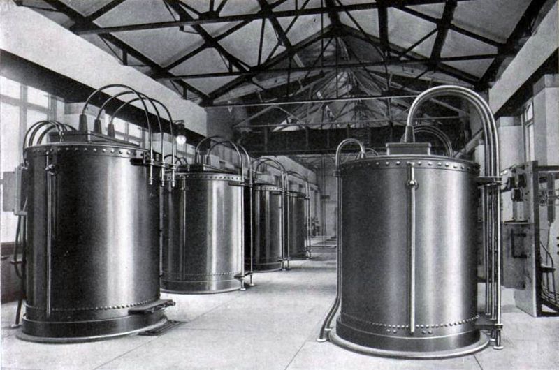
Transformers used for the Adams Power Plant Transformer House in Niagara Falls, which was built in 1895. Image in the public domain in the United States via Wikimedia Commons.
How Do Transformers Work?
Transformers have many different uses, but their basic design and operation remains the same. They typically consist of the following components:
- A ferromagnetic core, called E-, I-, U-, L-, toroidal, pot, or planar cores, depending on their shape
- Primary and secondary coils, also known as windings
When the device is connected to two (or more) circuits, it transfers the electrical current via electromagnetic induction. The primary winding receives the current, and the variations produce a magnetic field. Based on the ratio of turns in the windings, this field then generates either a higher, lower, or equal voltage in the secondary coil, thus making the turns ratio one of the main differences between step-up, step-down, and unity transformers.
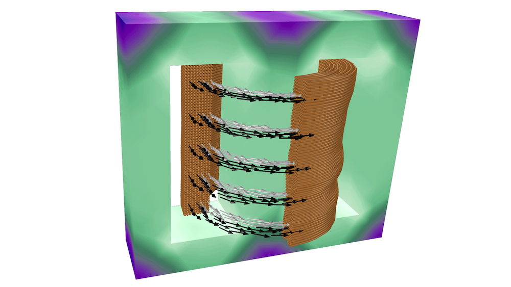
The magnetic fields in the core coupled to the currents in the windings for a unity transformer.
To improve the efficiency of a transformer, engineers need to analyze many different factors, such as the core’s ferromagnetic behavior (including resistance and magnetic saturation), the coupling between the magnetic and electric fields, and the number of windings. Using electromagnetics simulation, they can do just that using the COMSOL Multiphysics® software and add-on AC/DC Module. In the next section, you can take a look at a transformer example that has two different turns ratios: 1:1 for a unity transformer and 1000:1 for a step-down transformer.
Tip: If you prefer watching a video, we recommend this transformer simulation demonstration.
Modeling Transformers with the AC/DC Module
The two transformer models are set up in the same way (except for the turns ratio). There are two E-cores made of iron, and the windings are wrapped around the middle leg, as shown below. Placing the windings so close together (as opposed to, say, on separate legs) helps increase the magnetic coupling, making the transformer more efficient. To easily model these windings, you can use the built-in Coil feature. Note that here, the windings are assumed to be made of extremely thin wire, with a wire depth thinner than that of the skin depth.
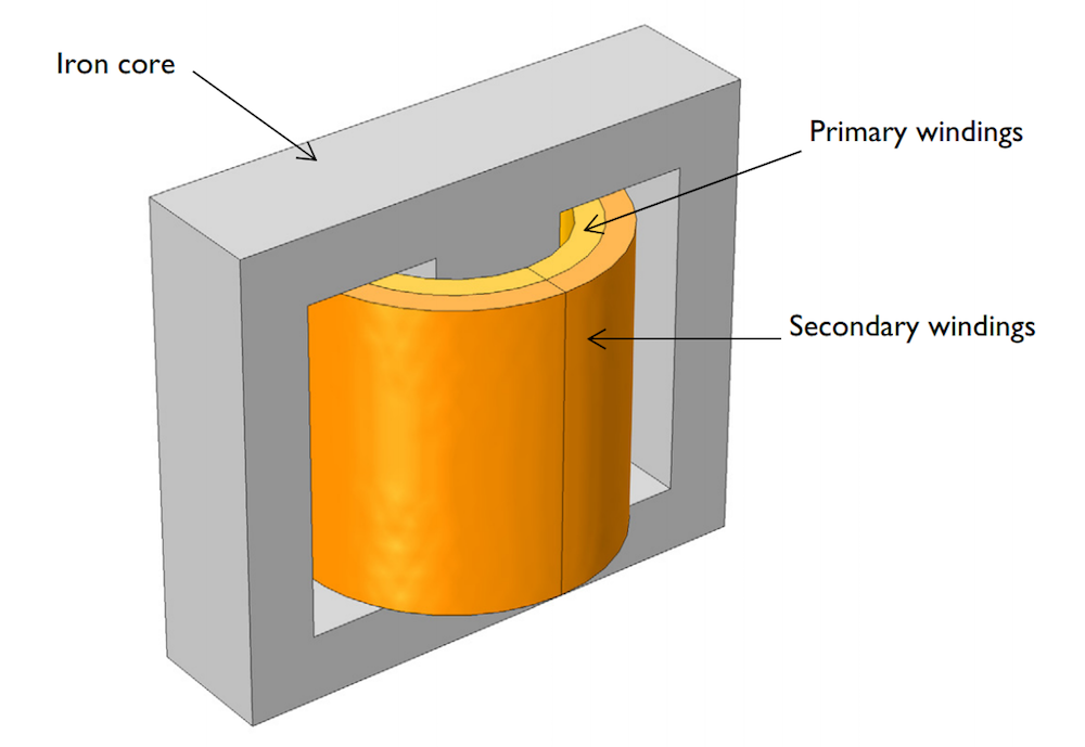
The geometry of an E-core transformer.
When modeling the iron cores, you can include the effect of the B-H curve (magnetic flux density versus magnetic field strength) using the Magnetic Fields interface. Adding in this curve helps capture the iron’s nonlinear behavior, enabling you to evaluate key factors, such as:
- Distribution of the magnetic and electric fields
- Transient response of the transformer
- Magnetic flux leakage
To streamline your analysis, you can parameterize key design factors, which makes them easy to alter and optimize. For instance, parameterizing the input voltage’s magnitude simplifies the process of ensuring that the number of windings is suitable for the voltage. Other parameters in this model include the line frequency (which is usually 50 Hz or, as in this case, 60 Hz); number of turns; and coil resistance.
In addition, you’re able to explore the effect of magnetic saturation, which dictates the maximum magnetic flux density in the transformer core. Since this is critical to performance, the saturation ends up limiting how small the core can be, which affects the cost. (The minimum size restriction is why you always see large transformers for high-power applications, like power plants.)
While we don’t go into detail about how to model the transformer in this blog post, you can find step-by-step instructions in the E-Core Transformer tutorial in the Application Gallery. Note that with a COMSOL Access account and valid software license, you can also download the MPH file for this example.
Examining the Unity and Step-Down Transformer Designs
To start, you can evaluate the unity transformer design at 50 ms. As the animation shows, the generated magnetic flux in the core is enough to induce voltages and currents in the windings, demonstrating that electromagnetic induction is achieved. These results are not only important to see if a design successfully transfers the input voltage but can also provide the insight needed to balance the transformer’s performance with its size and cost.
Magnetic flux density and currents in the core and windings, respectively.
Taking a closer look at the two coils, you can see that, as expected, the voltages are equal as a result of the turns ratios being equal. While the currents (shown below) are slightly different, this isn’t surprising, because the currents in the secondary coil are induced.


The currents in the primary (left) and secondary (right) winding for a unity transformer.
Moving on to the step-down transformer, you can see that this design successfully decreases the voltage by a factor of 1000 (from 25,000 V to 25 V).


The induced voltage in the primary (left) and secondary (right) winding for a step-down transformer.
As the results above show, you can evaluate the performance of different types of transformers via simulation, accurately accounting for electromagnetic and ferromagnetic effects. Using these results, engineers could improve the performance of transformer designs, optimizing them for specific applications.
Next Steps
Try it yourself: Download the E-core transformer tutorial by clicking the button below. Doing so will take you to the Application Gallery, where you can find documentation and the MPH file for this model.
You can also access a more advanced three-phase power transformer model that demonstrates how to compute electromagnetic quantities and losses in 3D and 2D-axisymmetric transformers.
Further Resources
- Watch a transformer simulation demo in the Transformer Design: A Multiphysics Approach video
- Learn about how ABB uses simulation to minimize transformer hum
- See how to model ferromagnetic materials


Comments (1)
TimothyaBigelow
September 22, 2020Model provided for E-core transformer does not run