
The Fraunhofer Institute for Nondestructive Testing (IZFP), headquartered in Germany, uses modeling and simulation in applied research focusing on the development of intelligent sensor and data systems for safety, sustainability, and efficiency. Sascha Thieltges of IZFP spoke with COMSOL about his team’s work in corrosion detection.
This blog post introduces a method for detecting corrosion in embedded pressure pipelines through guided waves excited by electromagnetic acoustic transducer (EMAT)-based systems. Get an introduction to the design challenges and risks associated with these pipeline systems, as well as the underlying analytical and numerical considerations. The blog post then demonstrates the analysis of a guided wave modeling problem in the COMSOL Multiphysics® software.
Early Corrosion Detection: A Key to Sustainable Infrastructure
Pipelines for energy distribution, water supply, and industrial processing form the backbone of modern infrastructure. Most of these systems were installed in the second half of the 20th century and are now increasingly affected by aging, mechanical stress, and environmental degradation (Ref. 1). One of the most critical failure mechanisms is corrosion-induced wall thinning, which can remain undetected until it results in structural failure (Ref. 2–4).
The earlier such degradation is identified, the more efficiently and cost-effectively maintenance can be planned. From an environmental perspective, early detection is equally important. Studies predict that by 2030, CO2 emissions from replacement steel production for corroded infrastructure could account for up to 5% of total global steel-related emissions (Ref. 5). Climate change further aggravates the issue, as extreme weather events occur more frequently, imposing growing stress on aging and insufficiently monitored systems.
Traditional inspection methods such as visual examinations or localized ultrasonic testing are limited when applied to embedded, insulated, or otherwise inaccessible pipeline sections, as shown in the photographs below. To reliably assess the internal condition of such systems, advanced nondestructive testing (NDT) methods are required; techniques that can probe long distances without direct surface access.

Difficult-to-access pipes under a bridge (left) and a pressure pipe embedded in concrete (right).
Guided ultrasonic waves address this need. They can propagate over several meters, interact with material discontinuities, and reveal early signs of corrosion. At the Fraunhofer Institute for Nondestructive Testing (Fraunhofer IZFP), a project team led by Sascha Thieltges is developing and advancing this approach to enable reliable condition monitoring, even under harsh and constrained conditions.
Hidden Risks in Embedded Pressure Pipelines
One of the most demanding applications of nondestructive testing is the inspection of embedded pressure pipelines, such as those used in alpine hydropower plants or long-distance supply systems. In these installations, a tunnel is excavated through solid rock, and a large-diameter steel pipe — typically between 800 mm and 3 m in diameter — is placed inside. The space between the pipe and tunnel wall is then filled with concrete to ensure structural integrity and load transfer. The end of such a pipe system is shown below.
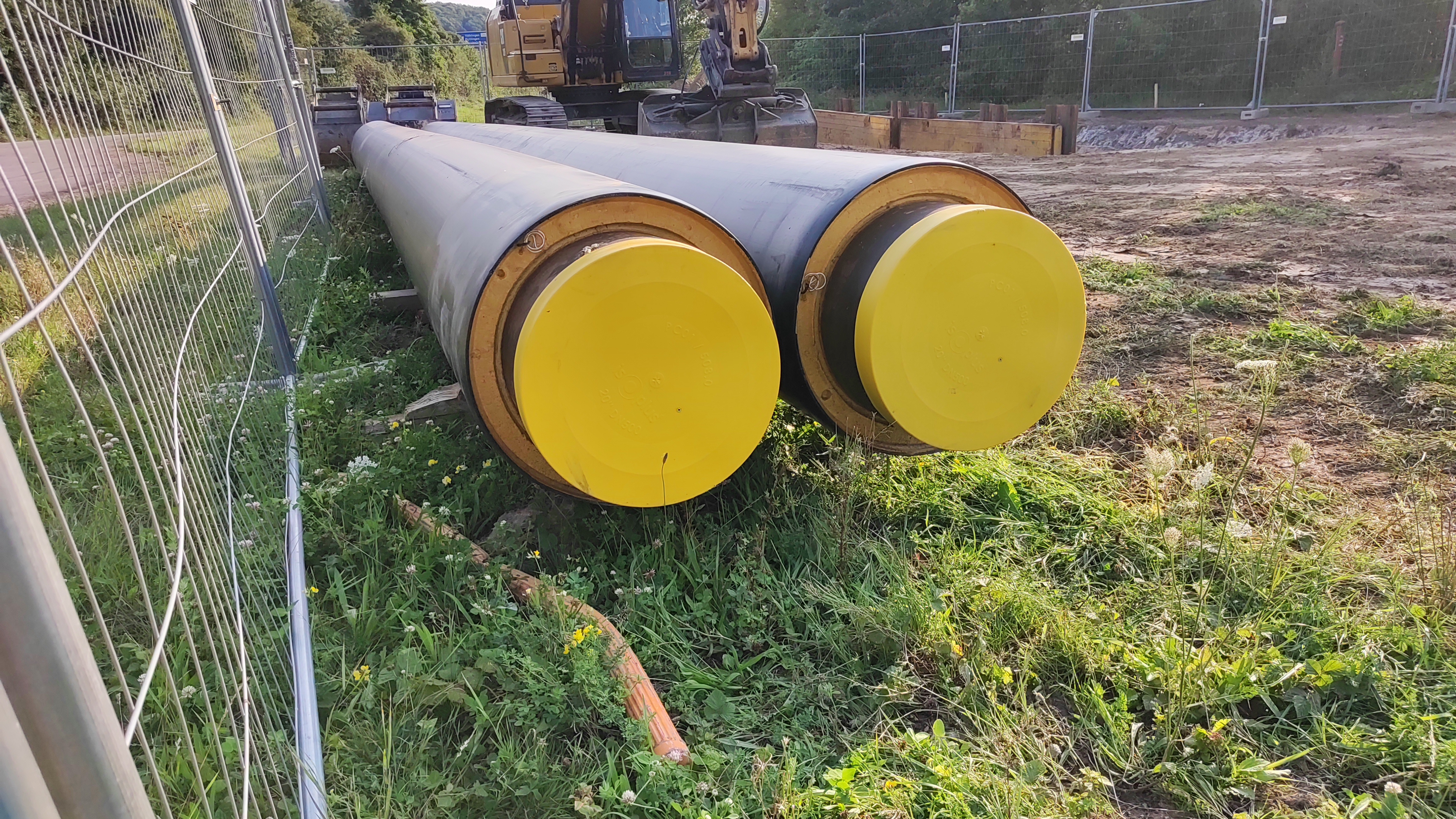 A district heating pipeline embedded in insulation.
This construction method presents a hidden risk: Water ingress through microcracks in the surrounding rock can accumulate along the pipe’s outer surface, causing localized external corrosion over time. Because these pipes often extend for several hundred meters, manual inspection is not feasible. “Conventional piezoelectric ultrasound only provides localized information — it simply doesn’t scale to full coverage,” explains Thieltges.
The key challenge is clear: How can the condition of such pipes be assessed when the outer surface is inaccessible and only short inspection windows are available from the inside? During scheduled shutdowns, the pipe is drained, cleaned, and inspected visually along with spot ultrasonic measurements. However, performing a full wall thickness mapping along the entire length is not practical due to the cost of downtime. “Any outage directly affects operations and revenue,” emphasizes Thieltges.
This is precisely where guided waves (GW) in combination with electromagnetic ultrasonic testing (EMUS) prove valuable. Guided waves can propagate several meters along the pipe while probing the full wall thickness. Electromagnetic acoustic transducer (EMAT)-based systems generate these waves without physical contact or coupling media — a critical advantage in embedded or harsh environments.
The Solution: GW Excited by EMATs
Among the various guided wave families, shear horizontal (SH) modes have shown promise for pipeline inspection (Ref. 6). These modes emerge as eigenmodes of the elastodynamic wave equation under boundary conditions representative of plate-like or cylindrical geometries. Rather than a single solution, a discrete set of modes exists, each characterized by a unique displacement profile across the wall thickness.
The displacement fields of odd and even modes can be expressed as:
(1)
(2)
with
(3)
where d_0 is the wall thickness, n is the mode index, and A_0 is the excitation amplitude.
Equations 1–2 describe a shear horizontal guided wave polarized in the x direction, propagating in the y direction, and exhibiting a sinusoidal or cosinusoidal amplitude distribution along the z axis.
The plot below illustrates the mode shapes for SH_0, SH_1, and SH_2 across the wall thickness. While SH_0 exhibits a uniform lateral displacement profile, higher modes such as SH_1 and SH_2 introduce depth-dependent motion, leading to increasingly complex propagation characteristics.
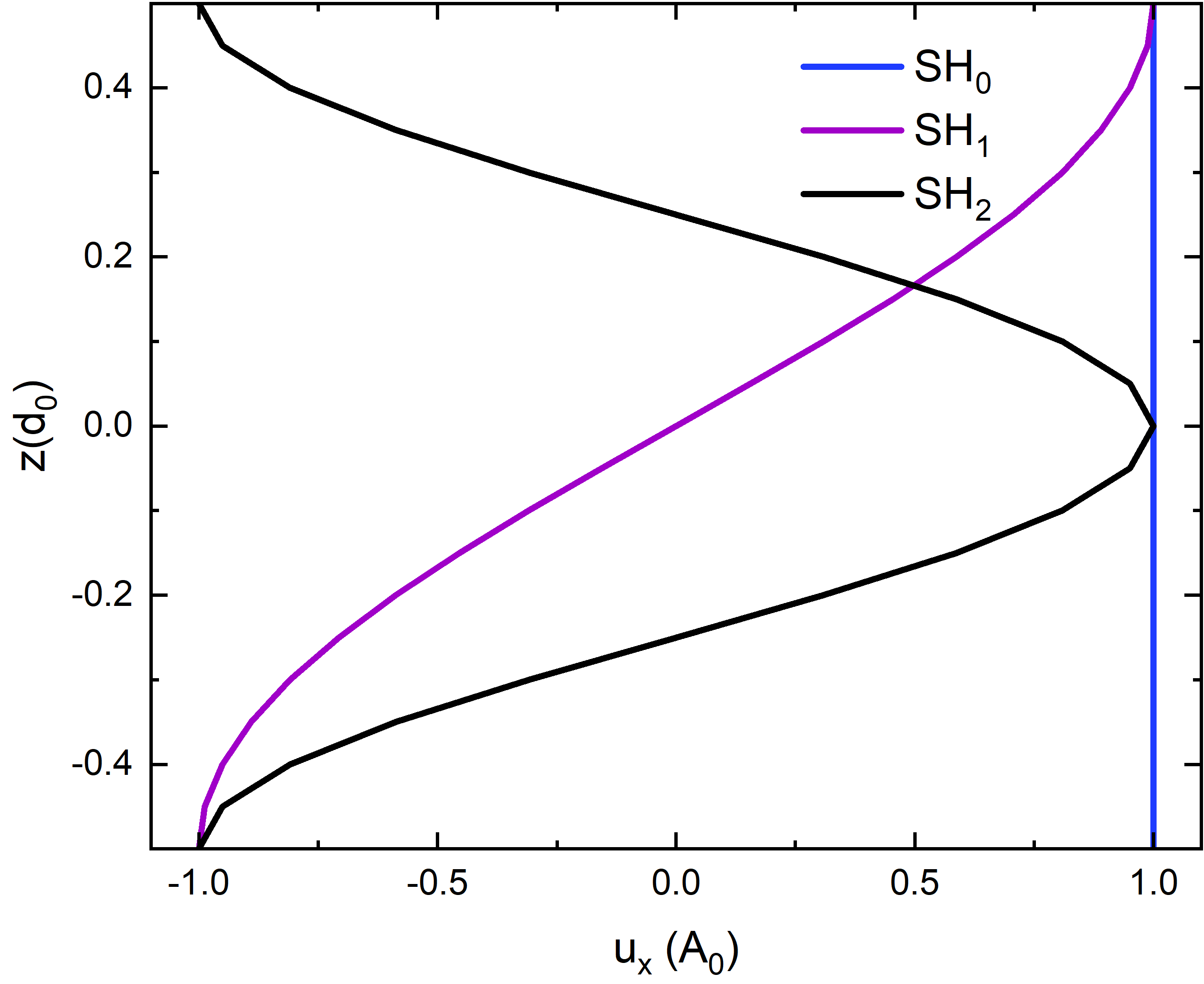 Distribution of the deflection amplitude of the SH0, SH1, and SH2 modes across the cross section.
A defining property of higher-order SH modes (n>0) is their dispersive nature. Both phase velocity c_P and group velocity c_G vary as functions of excitation frequency f and wall thickness d_0:
(4)
(5)
where c_T is the transverse wave velocity.
The plot below presents the dispersion curves (Eqs. 4–5) with representative operating points highlighted at wavelengths of 32 mm and 24 mm. Only guided waves that lie on the dispersion curves are physically supported, meaning that both wavelength and frequency must be carefully selected.
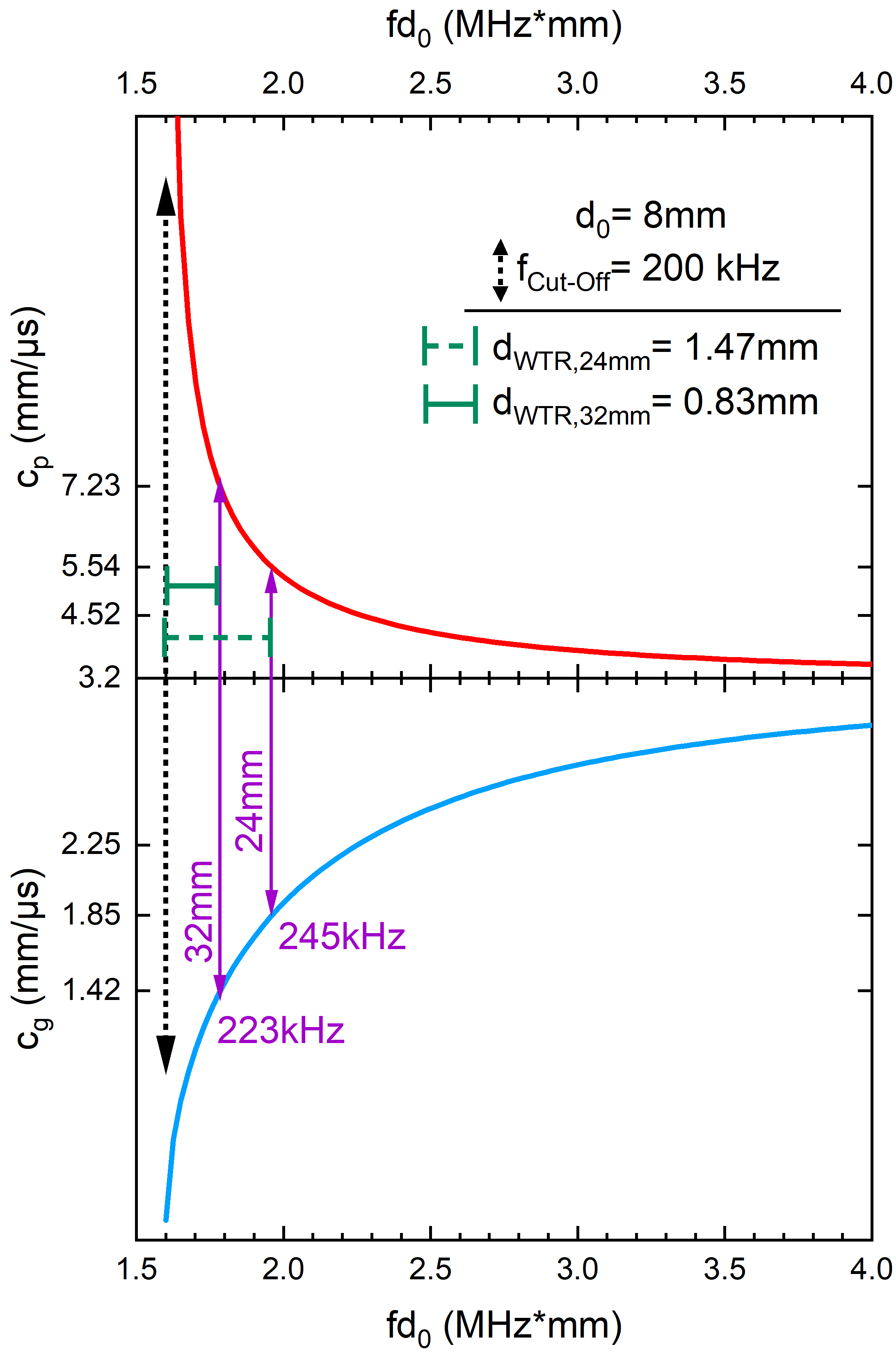 Dispersion curves according to Eqs. 4-5. Operating points for a GW with wavelengths of 32 mm and 24 mm are plotted in purple.
For a wall thickness of d_0=8mm, this corresponds to excitation frequencies of 223kHz (for \lambda=32mm) and 245kHz (for \lambda=24mm). If the wall thickness varies along the propagation path, the operating point shifts along the dispersion curve, altering both c_P and c_G.
For increasing wall thickness, both velocities asymptotically approach 3.2mm/µs (SH_0 mode). For decreasing wall thickness, however, the shifting of the operating point is limited. Below a critical wall thickness reduction (WTR), guided waves of the given wavelength can no longer propagate. For \lambda=24mm, the maximum wall thickness reduction is d_{WTR,24mm}=1.47mm, whereas for \lambda=32mm, the limit is d_{WTR,32mm}=0.83mm.
In practice, corrosion typically introduces localized reductions in wall thickness. These act as scattering centers, producing partial reflection of the guided wave. The reflection amplitude depends on the defect geometry, the selected wavelength, and the propagating mode. If the local wall reduction exceeds the permissible d_{WTR}, mode conversion occurs within the defect region, and the reflected signal may contain multiple mode components. “The sensor design is crucial here. It defines the operating point and thus directly determines which corrosion scenarios can be detected,” explains Thieltges.
The required excitation is provided by EMATs. An EMAT consists of high-frequency (HF) coils for excitation and reception, combined with a low-frequency static magnet. A high-frequency current (up to 50A peak-to-peak above 100kHz) in the coil generates a dynamic magnetic field. In the presence of the static field, Lorentz forces — or magnetostrictive forces, depending on the material — act at the surface and launch the guided wave. The operating principle is shown schematically below. The offset arrangement of RF coils (blue and green) relative to the static magnetic field (black arrow) enables unidirectional excitation of guided waves (red arrow).
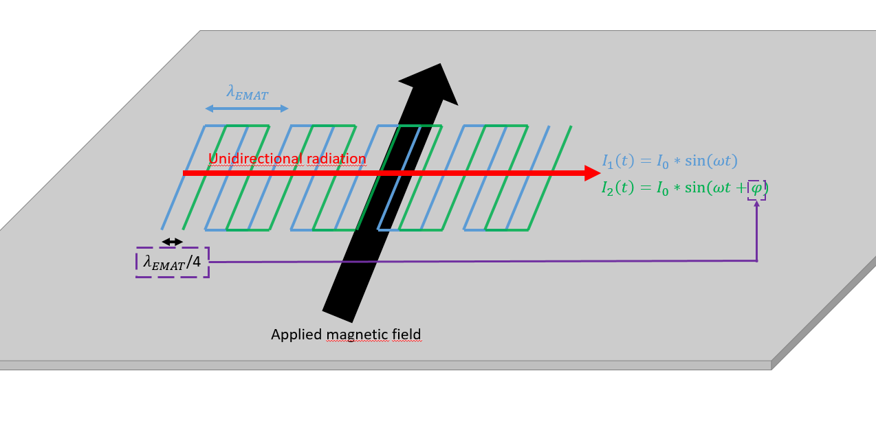 Schematic operating principle of an EMAT.
Guided waves, when excited and received in this manner, provide a versatile basis for corrosion detection and quantification. However, designing an effective EMAT-based inspection system remains a highly nontrivial task.
The key technical challenges at this stage of the modeling process can be summarized with the following questions:
- How can the coil geometry be optimized to achieve narrow-beam, unidirectional excitation?
- How can the wave amplitude be maximized, e.g., by enhancing Lorentz or magnetostrictive couplings?
- Which mode and operating point in the dispersion diagram are most sensitive to a given defect scenario?
- How do guided waves interact with corrosion sites in terms of reflection, attenuation, and mode conversion?
- How do surrounding media such as concrete or insulation alter wave propagation (e.g., through leaky-wave coupling) and how can these effects be mitigated?
Simulation as a Key Tool: Guided Wave Analysis in COMSOL Multiphysics®
Fully resolving the EMAT sensor, including coil design and coupled electromagnetic interactions, would be computationally prohibitive in this context. As a first step, a simplified model was therefore chosen, focusing exclusively on wave propagation and the interaction of guided waves with localized wall-thickness reductions in concrete-embedded pipes. “This is where simulations come into play, as they allow us to systematically investigate specific open questions,” explains Thieltges.
Instead of explicitly modeling the EMAT, its effect was represented through prescribed surface forces, applied as line loads on the inner pipe surface. Since shear-horizontal guided waves traverse the full wall thickness, the excitation side (inside or outside) is inconsequential. “By adjusting the spacing and temporal phasing of these loads, we were able to selectively excite either the SH_0 or SH_1 mode and analyze their reflection and scattering behavior at wall-thickness reductions. This abstraction isolates the key physical effects while keeping the computational cost manageable,” adds Thieltges.
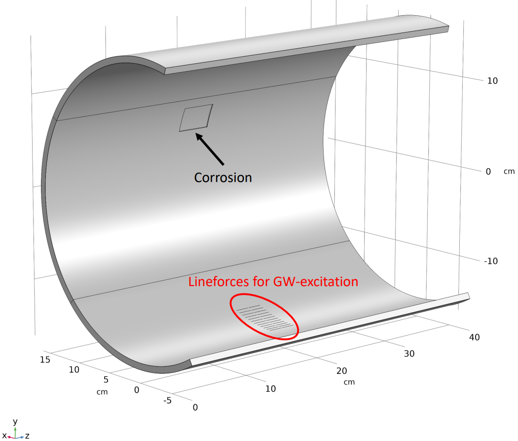
To achieve unidirectional wave excitation, four individual segments of line forces were implemented, each spatially offset and temporally phase shifted, as illustrated in the image below. Because the wave field is directed, the pipe geometry can be reduced, with low-reflecting boundary conditions applied in the circumferential direction to suppress spurious edge reflections. The model was constructed in full 3D and solved using the Structural Mechanics Module, an add-on to COMSOL Multiphysics®, in the time domain (transient analysis).
Accurate representation of guided wave phenomena requires particular care with spatial and temporal resolution. Both the mesh size and time step must be chosen to resolve the shortest wavelengths present and to minimize numerical dispersion. For practical guidance on mesh discretization and solver strategies in guided wave simulations, see COMSOL’s Knowledge Base article (Ref. 7).
Reflection Behavior of SH0 and SH1 Modes
The simulated pipe has a diameter of 323 mm and a nominal wall thickness of d_0=7.1mm. The wall thickness reduction (WTR) was varied between 5% and 90% of the nominal thickness, while both the SH0 (160 kHz) and SH1 (277 kHz) modes were selectively excited. To monitor the guided wave response, a point probe was placed on the outer pipe surface between the excitation region and the corrosion site, recording the displacement amplitude in the z direction over time.
The animation at left below illustrates the propagation and interaction of the SH₀ mode with a corrosion-induced WTR of 80%, while the animation at right below shows the SH₁ mode interacting with a localized WTR of 15%.
The time-domain signals (A-scans) obtained from the point probe are presented in the group of plots shown below. For each mode, the upper trace corresponds to the defect-free case (WTR = 0%), the middle trace to a corroded case (WTR = 25%), and the lower trace to the difference between both signals. This subtraction procedure suppresses the through-transmission component and isolates the reflection caused by the defect, making the reflected signal clearly visible.

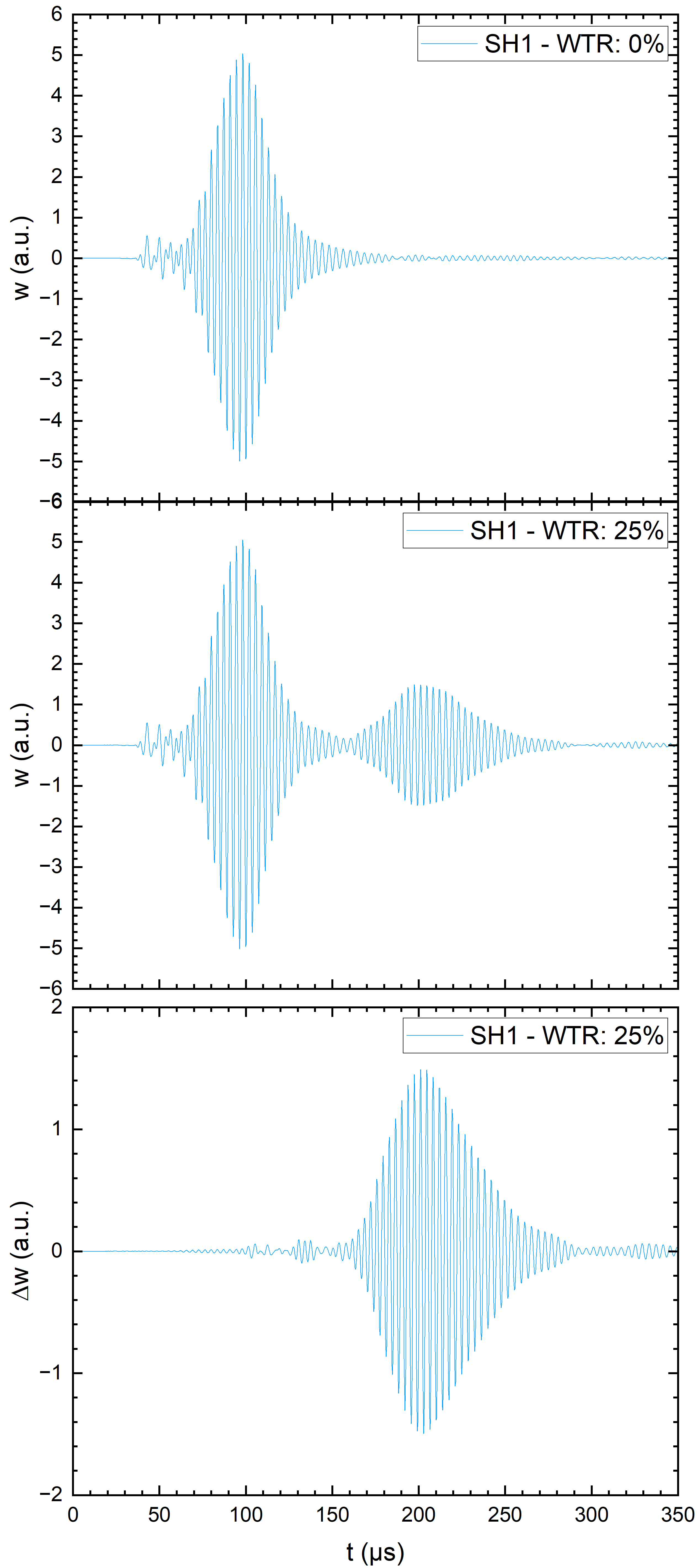
A-scans determined by spot sampling for the SH0 mode. Top left: WTR = 0%; center left: WTR = 25%; bottom left: difference between the two upper curves to highlight the reflection component. Top right: WTR = 0%; center right: WTR = 25%; bottom right: difference between the two upper curves to highlight the reflection component.
The dependence of the reflection amplitude on the WTR is summarized in the plot below. A distinct difference emerges between the two modes. At small WTR values below approximately 25%, the SH1 mode exhibits higher sensitivity, producing stronger reflections compared to the SH0 mode. Beyond this range, however, the reflection amplitude of SH1 decreases, while the SH0 mode exhibits an almost linear increase with defect depth.
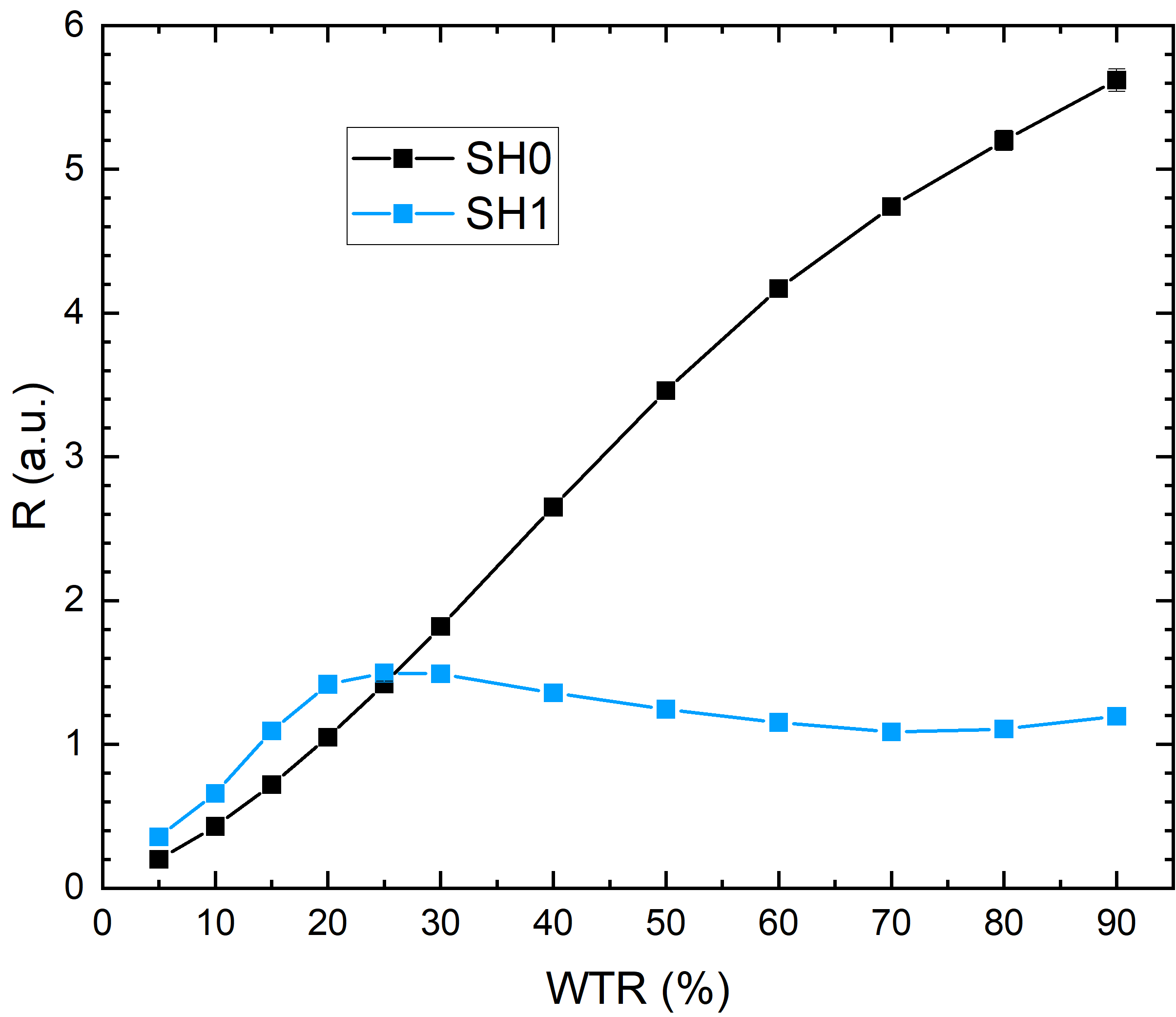 Reflection amplitudes for the SH0 and SH1 modes.
By contrast, the SH1 mode is dispersive and exhibits a depth-dependent displacement profile. As the local wall thickness approaches the propagation cutoff (d_{WTR,20mm} = 1.32 mm ↔ 18.6%), the effective coupling to the defect decreases, leading to reduced reflection amplitudes. In fact, simulations reveal that the SH1 mode cannot propagate through defects exceeding ~18.6% WTR. In such cases, mode conversion occurs within the defect region, redistributing energy into other guided modes.
These findings underscore a complementary sensitivity range. SH1 provides high sensitivity for detecting early-stage corrosion with small WTR, whereas SH0 maintains robust detectability for deeper WTR. The simulations therefore not only reproduce experimental observations but also offer a detailed physical explanation of the underlying mechanisms.
Perspective: From Surface Force Model to Complete EMAT-GW Modeling
The simulations presented here have deliberately relied on a simplified excitation model, where the physical effects of an electromagnetic–ultrasonic coupling were replaced by prescribed surface forces. This abstraction enabled an efficient and systematic study of guided-wave propagation, dispersion characteristics, and defect sensitivity. Even in this reduced form, the simulations yielded valuable insights: They demonstrated the complementary detection ranges of SH0 and SH1 modes, highlighted the dependence of reflection behavior on WTR, and confirmed the potential of guided waves for early corrosion detection in embedded pipelines.
The key advantage of this approach lies in its efficiency. By decoupling the excitation mechanism from the propagation problem, it becomes possible to focus computational resources on the interaction of guided waves with structural variations. This has already provided a physics-based rationale for mode selection, excitation frequency, and defect detectability: parameters that directly guide sensor development and testing strategies.
The next step, however, is to expand the model toward a complete physical representation of the EMAT sensor. In this extended framework, both the coil geometry and the static magnetic field will be explicitly modeled, together with the Lorentz and magnetostrictive forces that give rise to guided-wave excitation. Incorporating these mechanisms will make it possible to realistically predict the energy input, capture the true radiation characteristics of the wave field, and optimize the sensor design for specific defect scenarios.
By bridging the gap between simplified force-based excitation and fully coupled EMAT simulations, this approach paves the way for digital prototyping of guided-wave systems. Such models will not only reduce experimental trial-and-error but also accelerate the design of robust, application-specific EMAT solutions for nondestructive testing under challenging conditions.
About the Guest Author
Sascha Thieltges is a physicist and scientific researcher at the Fraunhofer Institute for Nondestructive Testing (IZFP), where he is currently pursuing his doctoral studies. His work focuses on the development and application of electromagnetic nondestructive testing methods, including EMAT, 3MA, and ferromagnetic hysteresis measurements. A central aspect of his research is the multiphysical modeling of these techniques, bridging experimental investigations and numerical simulation. In addition, he serves as a project lead for applied research projects in the field of material characterization and condition assessment.
References
- PwC and Oxford Economic, “Global Infrastructure Outlook – Infrastructure investment needs 50 countries, 7 sectors to 2040”.
- Thakur et al., “Chapter 1: Understanding the Chemistry and Common Issues of Infrastructure Corrosion,” Architectural Corrosion and Critical Infrastructure, 2025.
- Xu, “Corrosion is a global menace to crucial infrastructure — act to stop the rot now,” Nature, vol. 629, no. 41, 2024. doi.org/10.1038/d41586-024-01270-7.
- Li, “Materials science: Share corrosion data,” Nature, vol. 527, pp. 441–442, 2015. doi.org/10.1038/527441a.
- S. F. M. Iannuzzi, “The carbon footprint of steel corrosion,” npj Mater Degrad, vol. 6, no. 101, 2022. doi.org/10.1038/s41529-022-00318-1.
- L. Rose, Ultrasonic Guided Wave in Solid Media, Cambridge University Press, 2014.
- COMSOL, “Resolving Time-Dependent Waves,” https://www.comsol.com/support/knowledgebase/1118.


Comments (0)