
Previously on the blog, we looked at setting up a programmatic sequence of operations under the Study node for solving, saving a model to file, and exporting data to file. In this blog post, we are building on this knowledge to show how an entire sequence of images can be automatically exported after solving a model in the COMSOL Multiphysics® software.
Editor’s note: The original version of this post was published on July 11, 2017. It has since been updated with new content and screenshots.
Example: Micromixer Model
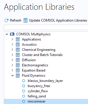
To demonstrate this functionality, just like in our previous blog post “How to Use Job Sequences to Save Data After Solving Your Model”, we will first load the Micromixer tutorial model from the Application Libraries. This model is available in the folder COMSOL Multiphysics > Fluid Dynamics and illustrates fluid flow and mass transport in a laminar static mixer.
The model performs a fluid flow simulation using a Laminar Flow interface. In the next step, it shows how to calculate the mixing efficiency by means of a Transport of Diluted Species interface, using the results from the fluid flow simulation as input. The species will be transported downstream based on the fluid velocity.
The computation time for this model is a few minutes. In the previous blog post, we made the computations go faster by not solving for the Transport of Diluted Species part. However, this time around, we will need the concentration profile throughout the mixer. To run the computation quicker in this case, you can set the Predefined Element Size to Extremely coarse.
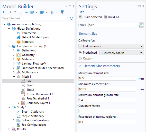
For this example, the step of coarsening the mesh is optional and everything that follows will work even without this change.
Let’s now see how to use a parameterized slice plot together with an animation to export an entire series of images, where each image corresponds to a single slice.
Using Parameters to Position a Slice Plot
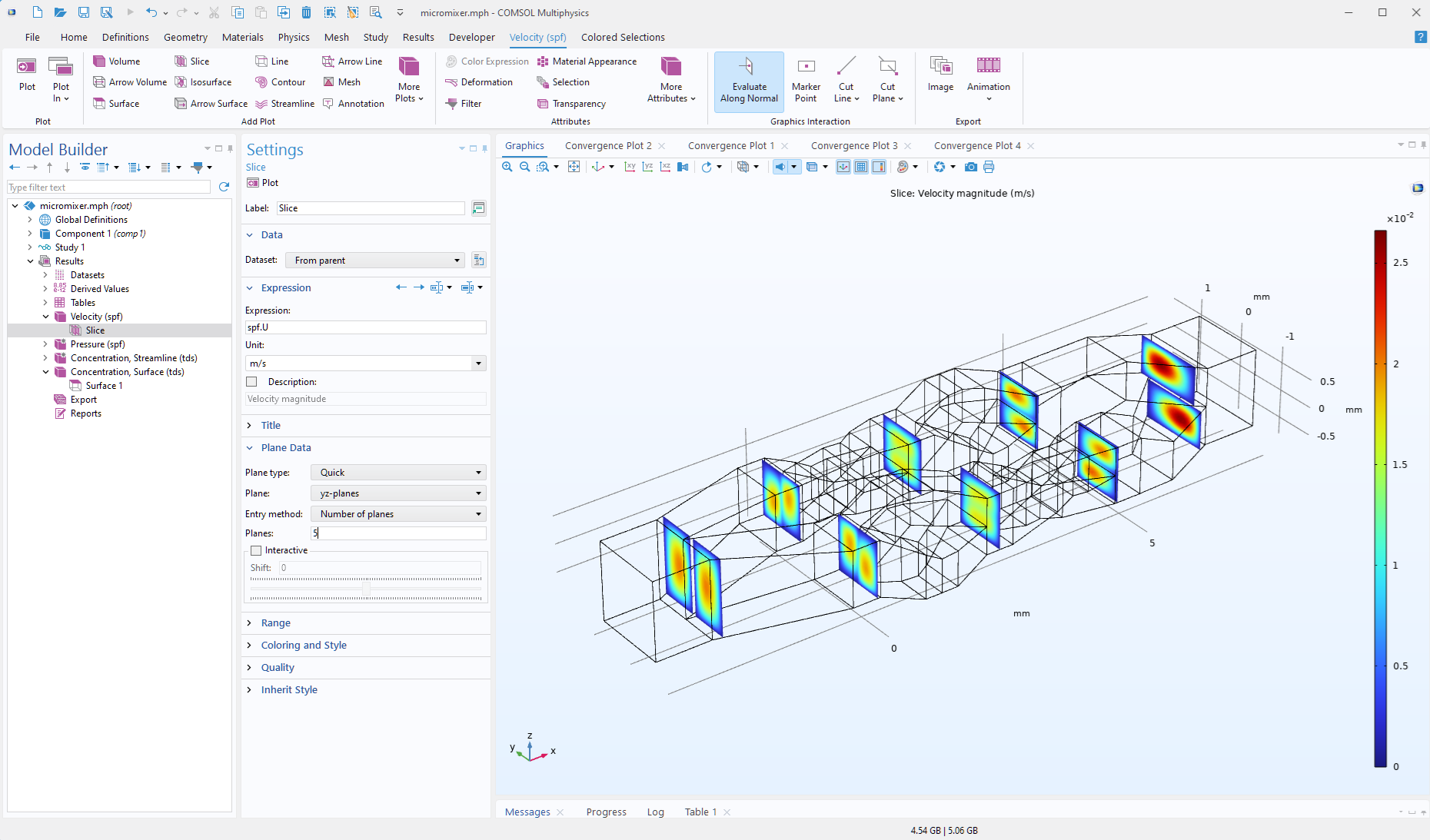
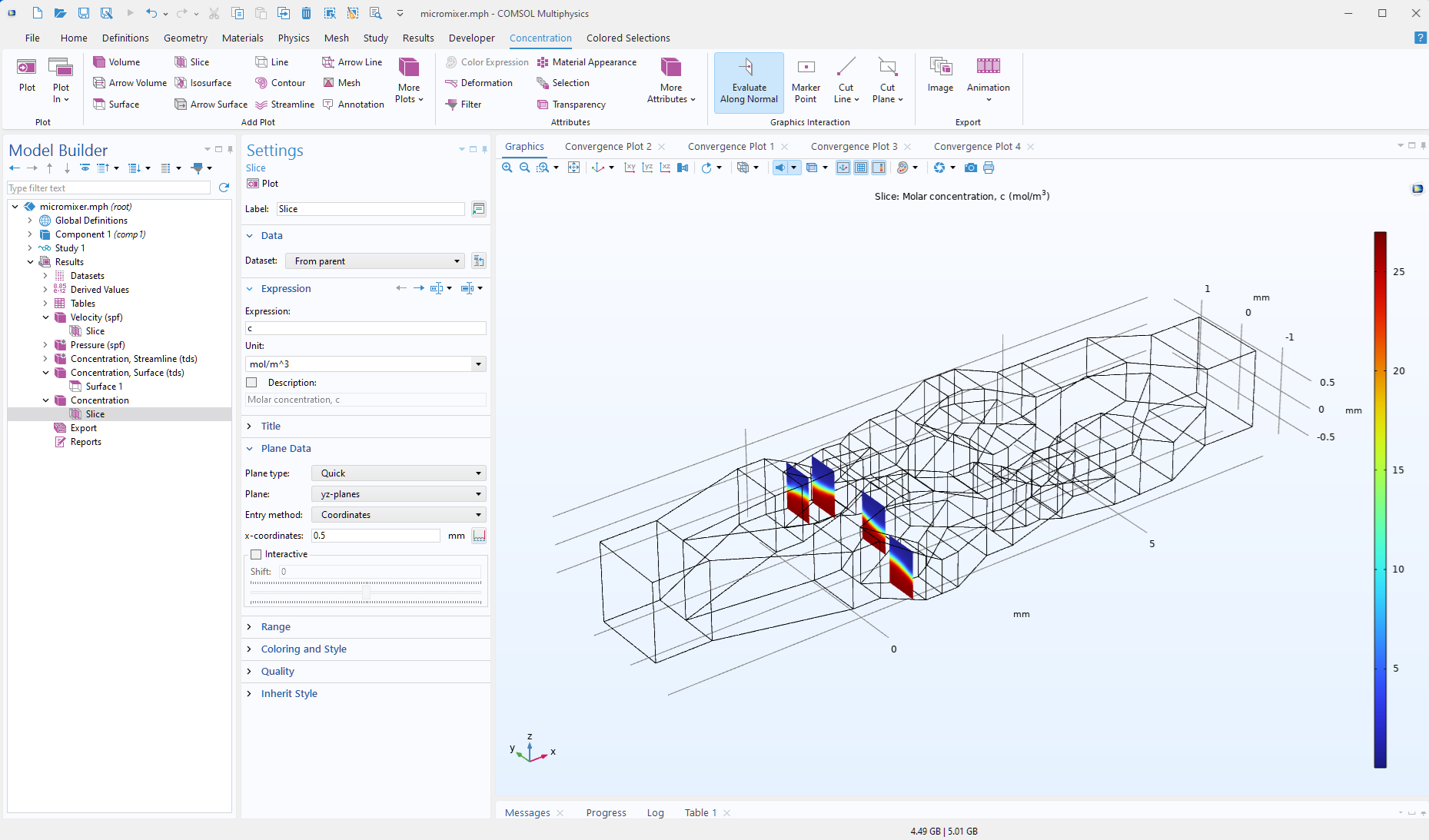
This is the default plot for the velocity at 5 different yz-plane slices in the x direction in a solved version of the library model:
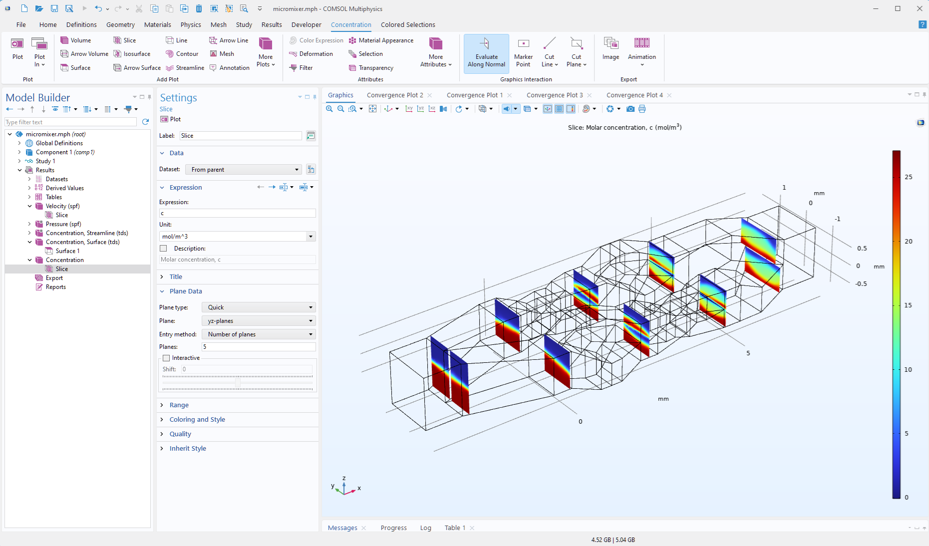
Let’s create a similar slice plot but for the concentration. Right-click the Velocity (spf) node and select Duplicate. In the newly created plot group, change the name to Concentration and the Expression to c for concentration:
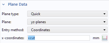
Instead of the default 5 evenly spaced slices in the Slice plot for the Concentration, you can change the Plane Data entry method to Coordinates. For example, you can generate a single slice at 0.5 mm, as follows.
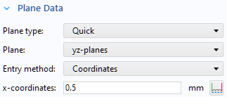
The resulting plot is shown in the figure below:
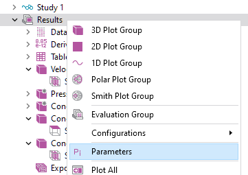
We can parameterize the location of the slices by means of a Results Parameter. Right-click the Results node and select Parameters.
Define a parameter xcut with the value -3.5[mm]. (The microchannel ranges from -3.5 mm to 8 mm in the x direction.)
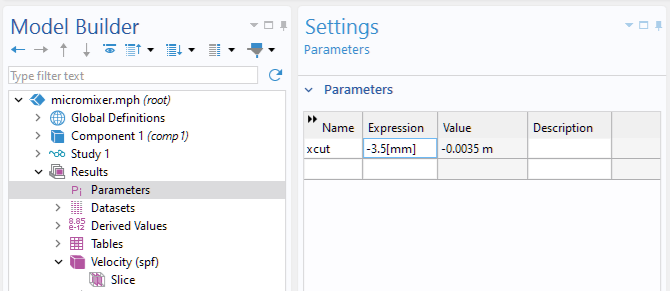
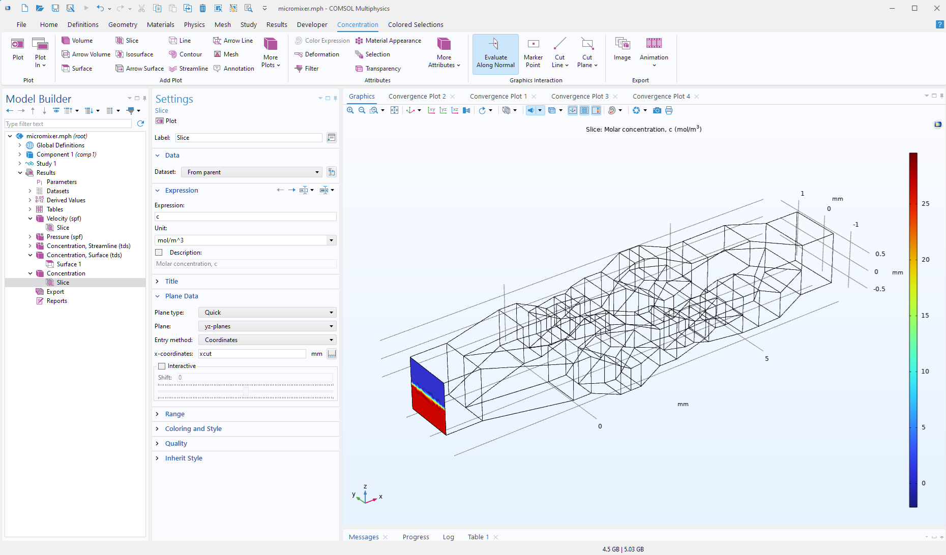
For the Slice plot for Concentration, in the section for Plane Data, type xcut in the edit field for x-coordinates.
The corresponding slice plot is shown here:
Using an Animation to Export a Sequence of Images
What if you would now like to export a series of images corresponding to different values of the slice position? For this purpose, you can use a file-export-based animation.
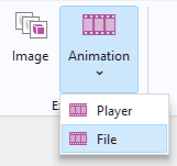
To generate an animation, select File from the Animation menu in the ribbon toolbar.
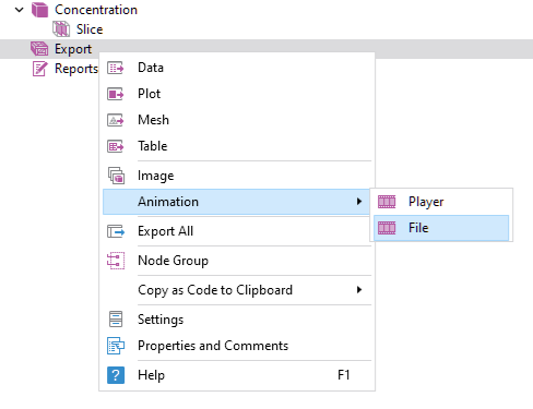
Alternatively, you can right-click the Export node under Results and select Animation > File.
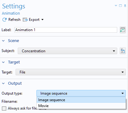
In the Settings window for the Animation node in the model tree, change the Subject to Concentration. Then, select Image sequence as the Output type.
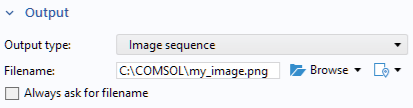
For the Filename, type, for example, C:\COMSOL\my_image.png. This assumes that you have a folder C:\COMSOL in your system, but you can write to any folder where you have write permission.
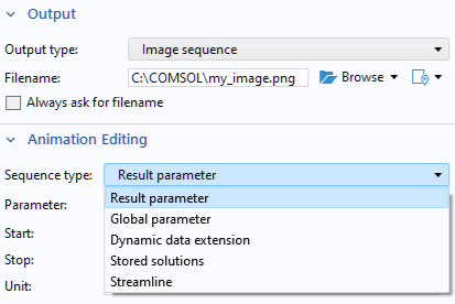
To link the exported file to the parameter xcut, change the Sequence type to Result parameter. This setting is available in the Animation Editing section.
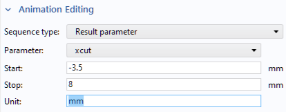
Choose xcut as the Parameter, with Start set to -3.5, Stop set to 8, and Unit set to mm.
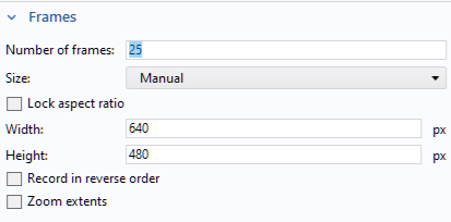
At the top of the Animation settings window, click Export to start the generation of images. The images will get a suffix corresponding to the number in the sequence. The number of frames, or images, is set in the Frames section.
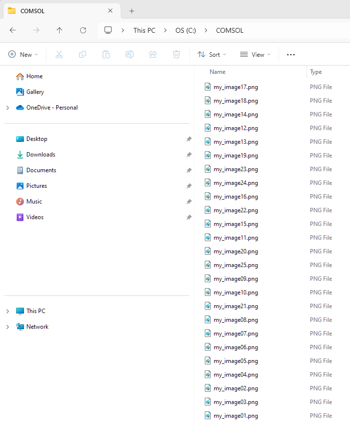
A series of images is generated with names: my_image01.png, my_image02.png, …, my_image25.png, as shown in the screenshot below.
Automatic Export After Solving the Model
Let’s now see how the generation of images can be made automatically after solving a model in COMSOL Multiphysics.
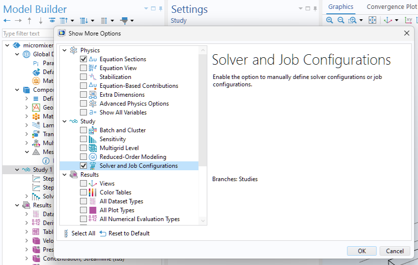
To be able to define a sequence of operations under the Study node, enable Solver and Job Configurations. This option is available in the Show More Options dialog available from the Model Builder toolbar. Click the “eye” icon to open the dialog.
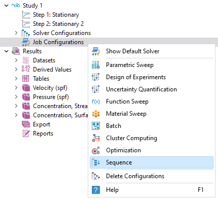
Under the Job Configuration node that is now visible, select Sequence. This procedure was described in the previous blog.
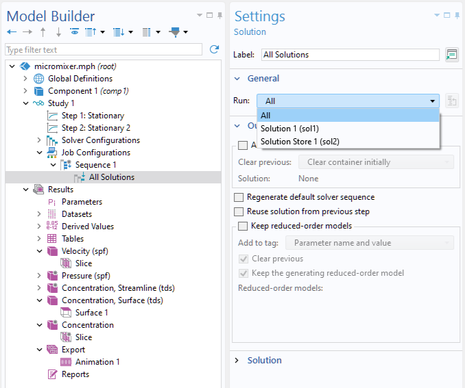
Right-click the Sequence and select Solution. In the Solution settings window, if not already selected, select All. This ensures that all study steps are run.
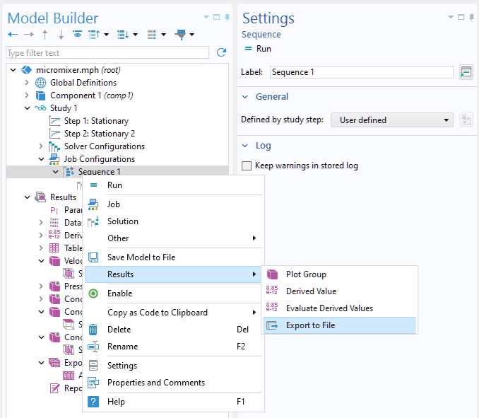
Right-click Sequence and select Results > Export to File.
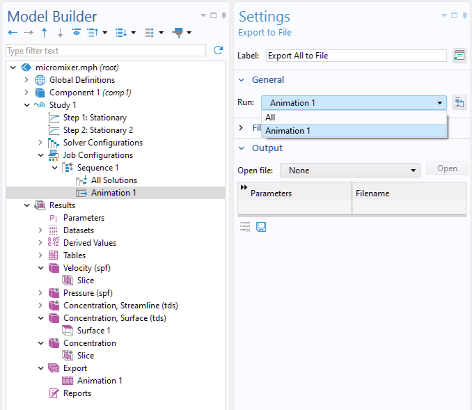
In the Export to File settings window, select Animation 1 under the Run option. In this simple example with just one node under Export, we could here just as well have left the default option All.
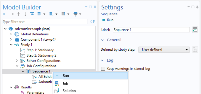
To solve using the Sequence, right-click and select Run. Alternatively, click the Run button at the top of the Sequence settings window. This will run the entire model again and when solved, export the image files.
Using Cut Planes to Export 2D Images
The previous export operation generated a series of 3D images. What if you want a series of 2D images for each slice? This can be accomplished by using a parameterized Cut Plane.
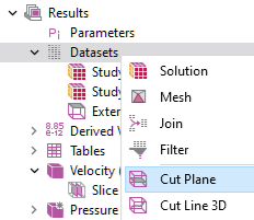
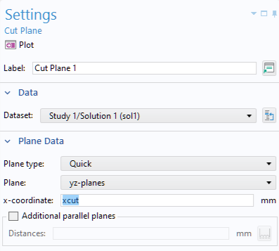
Right-click the Data Sets node and select Cut Plane.
In the Cut Plane settings window, type xcut for the x-coordinate.
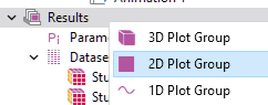
The already existing 3D plot groups are not useful for 2D plots, so right-click Results and select 2D Plot Group.
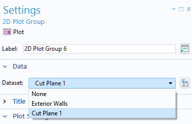
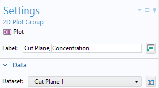
In the 2D Plot Group settings window, select Cut Plane 1 as the Data set.
Add a Surface plot node under the 2D Plot Group and change the Expression to c, corresponding to the concentration.
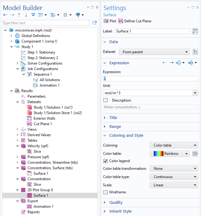
To tidy up the list of plot groups, change the name of the 2D Plot Group to Cut Plane, Concentration.
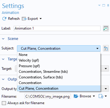
Now, go to the Animation node in the model tree. In the corresponding Settings window, change the Subject to Cut Plane, Concentration.
Click Export to generate the sequence of 2D images, as shown here in the file browser view:
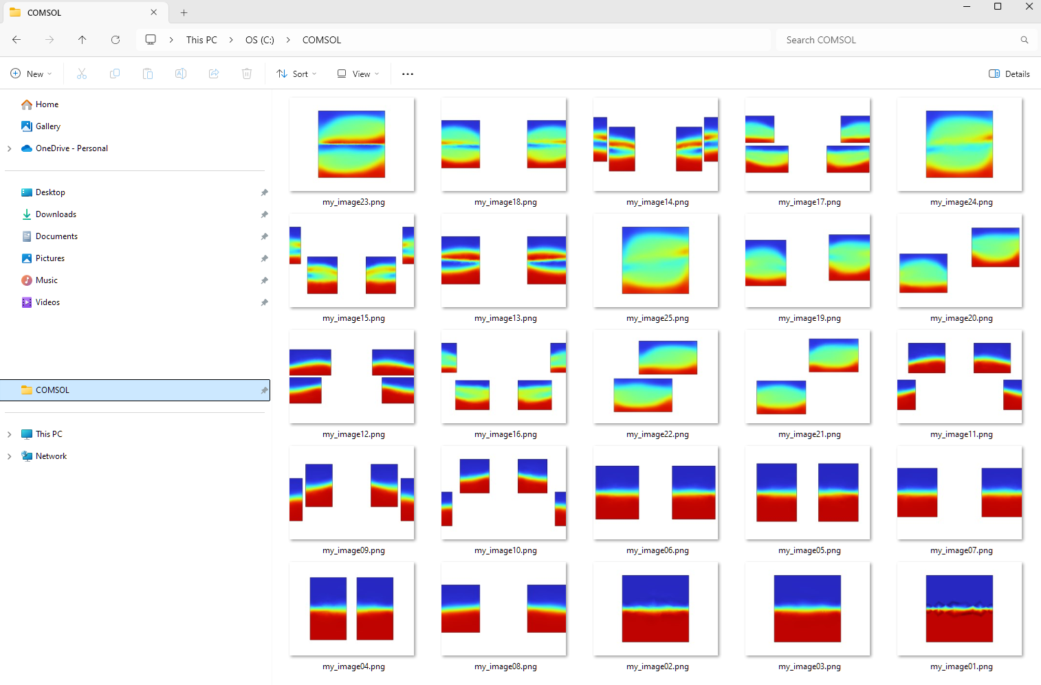
To get this view using Windows® Explorer, change the view to Large Icons.
Just like in the previous example, you can now go ahead and run the Job Sequence to solve and then have the set of images generated and saved to file — automatically.
Next Step
To try the example featured throughout this blog post yourself, click on the button below to access the MPH files.
Microsoft and Windows are either registered trademarks or trademarks of Microsoft Corporation in the United States and/or other countries.


Comments (0)