Designing MEMS devices, such as piezoresistive pressure sensors, comes with challenges. For instance, accurately describing the operation of these devices requires the integration of various physics. With the COMSOL Multiphysics® software, you can easily couple multiphysics simulations in order to test a device’s performance and generate reliable results. Today, we’ll look at one example that showcases such capabilities.
Piezoresistive Pressure Sensors “Measure Up” to the Competition
One of the first types of commercialized MEMS devices was the piezoresistive pressure sensor. This device, which continues to dominate the pressure sensor market, is valuable in a range of industries and applications. Measuring blood pressure as well as gauging oil and gas levels in vehicle engines are just two examples.
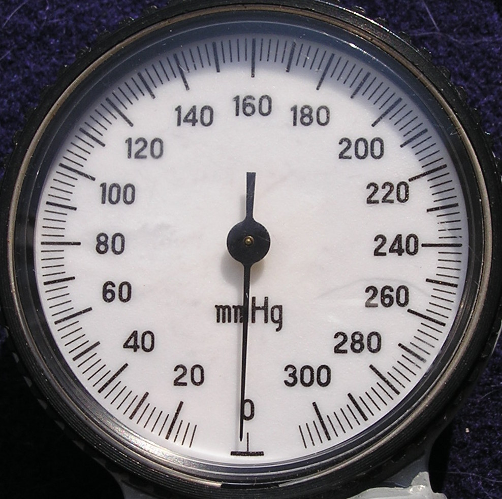

Piezoresistive pressure sensors have applications in the biomedical field as well as the automotive industry. Left: A blood pressure measurement device. Image by Andrew Butko. Licensed under CC BY-SA 3.0, via Wikimedia Commons. Right: A vehicle’s oil gauge. Image by Marcus Yeagley. Licensed under CC BY-SA 2.0, via Flickr Creative Commons.
While piezoresistive pressure sensors require additional power to operate and feature higher noise limits, they offer many advantages over their capacitive counterparts. For one, they are easier to integrate with electronics. They also have a more linear response in relation to the applied pressure and are shielded from RF noise.
But like other MEMS devices, piezoresistive pressure sensors include multiple physics within their design. And in order to accurately assess a sensor’s performance, you need to have tools that enable you to couple these different physics and describe their interactions. The features and functionality of COMSOL Multiphysics enable you to do just that. From your simulation results, you can get an accurate overview of how your device will perform before it reaches the manufacturing stage.
To illustrate this, let’s take a look at an example from our Application Gallery.
Evaluate the Performance of a Piezoresistive Pressure Sensor with COMSOL Multiphysics®
The design of our Piezoresistive Pressure Sensor, Shell tutorial model is based on a pressure sensor that was previously manufactured by a division of Motorola that later became Freescale Semiconductor, Inc. While the production of the sensor has stopped, there is a detailed analysis provided in Ref. 1 and an archived data sheet available from the manufacturers in Ref. 2.
Our model geometry is comprised of a square membrane that is 20 µm thick, with sides that are 1 mm in length. A supporting region that is 0.1 mm wide is included around the edges of the membrane. This region is fixed on its underside, indicating a connection to the thicker handle of the device’s semiconducting material. Near one of the membrane’s edges, you can see an X-shaped piezoresistor (Xducer™) as well as some of its associated interconnects. Only some interconnects are included, as their conductivity is high enough that they don’t contribute to the device’s output.
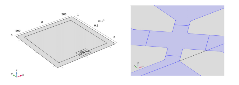
Geometry of the sensor model (left) and a detailed view of the piezoresistor geometry (right).
A voltage is applied across the [100] oriented arm of the X, generating a current down this arm. When pressure induces deformations in the diaphragm in which the sensor is implanted, it results in shear stresses in the device. From these stresses, an electric field or potential gradient that is transverse to the direction of the current flow occurs in the [010] arm of the X — a result of the piezoresistance effect. Across the width of the transducer, this potential gradient adds up, eventually producing a voltage difference between the [010] arms of the X.
For this case, we assume that the piezoresistor is 400 nm thick and features a uniform p-type density of 1.31 x 1019 cm-3. While the interconnects are said to have the same thickness, their dopant density is assumed to be 1.45 x 1020 cm-3.
With regards to orientation, the semiconducting material’s edges are aligned with the x– and y-axes of the model as well as the [110] directions of the silicon. The piezoresistor, meanwhile, is oriented at a 45º angle to the material’s edge, meaning that it lies in the [100] direction of the crystal. To define the orientation of the crystal, a coordinate system is rotated 45º about the z-axis in the model. This is easy to do with the Rotated System feature provided by the COMSOL software.
In this example, we use the Piezoresistance, Boundary Currents interface to model the structural equations for the domain as well as the electrical equations on a thin layer that is coincident with a boundary in the geometry. Using this kind of 2D “shell” formulation significantly reduces the computational resources required to simulate thin structures. Note that both the MEMS Module and the Structural Mechanics Module are used to perform this analysis.
Comparing the Results
To begin, let’s look at the displacement of the diaphragm after a 100 kPa pressure is applied. As the simulation plot below shows, the displacement at the center of the diaphragm is 1.2 µm. In Ref. 1, a simple isotropic model predicts a displacement of 4 µm at this point. Considering that the analytic model is derived from a crude variational guess, these results show reasonable agreement with one another.
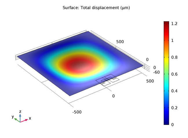
The displacement of the diaphragm following a 100 kPa applied pressure.
When using a more accurate value for shear stress in local coordinates at the diaphragm edge’s midpoint, the local shear stress is said to be 35 MPa in Ref. 1. This is in good agreement with the minimum value from our simulation study (38 MPa). In theory, the shear stress should be the greatest at the diaphragm edge’s midpoint.
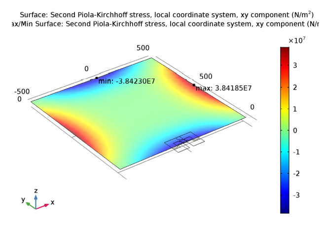
Shear stress in the piezoresistor’s local coordinate system.
The following graph shows the shear stress along the edges of the diaphragm. The maximum local shear stress of 38 MPa is at the center of each of the edges.
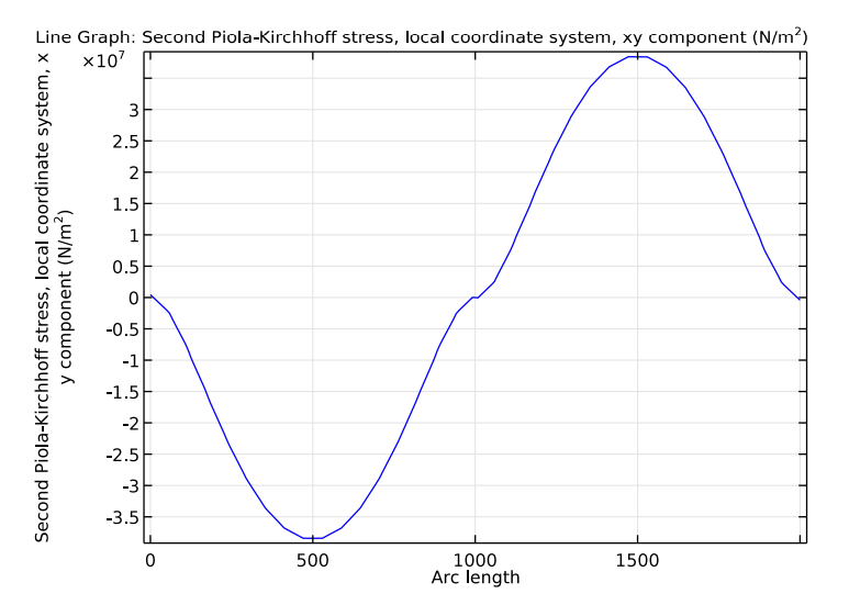
Local shear stress along two of the diaphragm’s edges.
Given that the dimensions of the device and the doping levels are estimates, the model’s output during normal operation is in good agreement with the information presented in the manufacturer’s data sheet. For instance, in the model, an operating current of 5.9 mA is obtained with an applied bias of 3 V. The data sheet notes a similar current of 6 mA. Further, the model generates a voltage output of 54 mV. As indicated by the data sheet, the actual device produces a potential difference of 60 mV.
Lastly, we look at the detailed current and voltage distribution inside the Xducer™ sensor. As noted by Ref. 3, a “short-circuit effect” may occur when voltage-sensing elements increase the current-carrying silicon wire’s width locally. This effect essentially means that the current spreads out into the sense arms of the X. The short-circuit effect is illustrated in the plot below. Also highlighted is the asymmetry of the potential, which is a result of the piezoresistive effect.
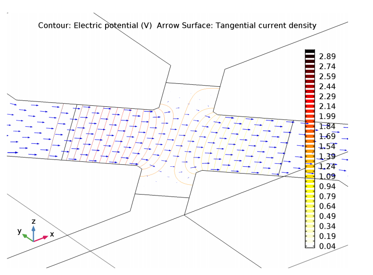
Current density and electric potential for a device with a 3 V bias and an applied pressure of 100 kPa.
Further Resources
- Get a demonstration of the Piezoresistive Pressure Sensor, Shell tutorial in this archived webinar
- Browse the MEMS category on the COMSOL Blog to learn more about simulation applications for MEMS devices
References
-
S.D. Senturia, “A Piezoresistive Pressure Sensor”, Microsystem Design, chapter 18, Springer, 2000.
-
Motorola Semiconductor MPX100 series technical data, document: MPX100/D, 1998.
-
M. Bao, Analysis and Design Principles of MEMS Devices, Elsevier B. V., 2005.
Xducer™ is believed to be a trademark of Freescale Semiconductor, Inc. f/k/a Motorola, Inc. Neither Freescale Semiconductor Inc. nor Motorola, Inc. has in any way provided any sponsorship or endorsement of, nor do they have any connection or involvement with, COMSOL Multiphysics® software or this model.


Comments (2)
James Ransley
December 28, 2016Just a brief note – in December 2015 Freescale Semiconductor was acquired by NXP Semiconductors, part of a wider pattern of consolidation in the semiconductor industry in the last few years.
James Ransley
December 28, 2016And a further brief comment – Qualcomm are actually in the process of acquiring NXP – if the deal is approved by regulators.