Self-driving cars have long been a staple of science fiction, but unlike other inventions dreamed up by speculative fiction writers, fully autonomous vehicles have come surprisingly close to becoming a reality over the past decade. In this blog post, learn how the COMSOL Multiphysics® software can be used to model lidar — a key technology enabling self-driving cars and autonomous robots to be aware of their surroundings.
Route to Fully Autonomous Vehicles
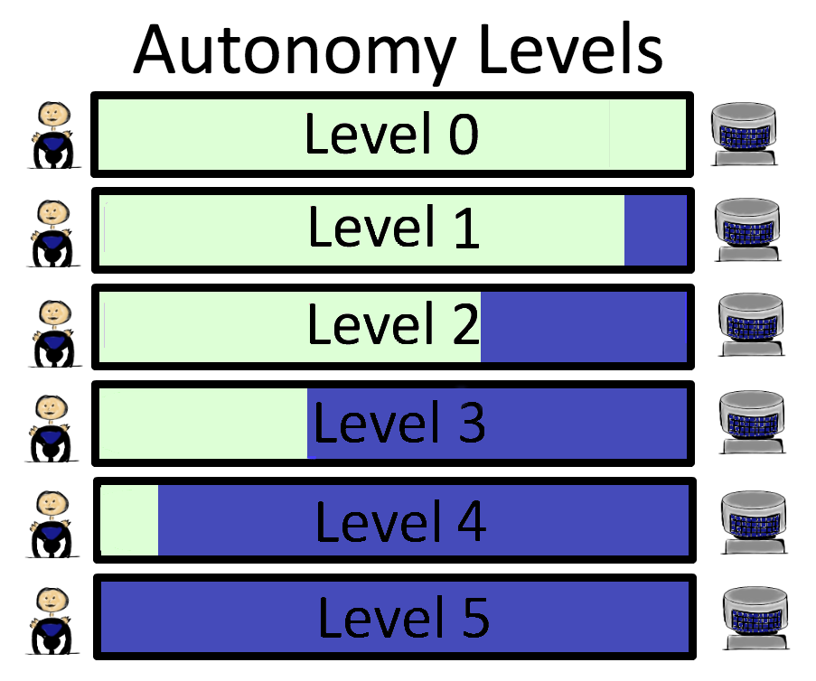
The industry standard for evaluating the autonomy of a vehicle was developed by the Society of Automotive Engineers (SAE). Its six levels of automation (starting with level 0) are categorized based on which dynamical driving tasks (DDTs) can be performed by the machine and which tasks need human involvement:
- Level 0: No automated driving; the human driver performs all DDTs for the vehicle
- Level 1: Automated assistance for either steering or acceleration and deceleration (e.g., cruise control); the human driver performs all other DDTs for the vehicle
- Level 2: Automated assistance for steering and acceleration and deceleration (e.g., automated parallel parking); the human driver performs all other DDTs
- Level 3: Automated DDTs for the vehicle; the human driver closely monitors the car and intervenes if necessary
- Level 4: Automated DDTs for the vehicle; the human driver does not need to intervene
- Level 5: Completely automated DDTs; the human driver does not have to be in the front seat
 An illustration showing the six levels of autonomous driving described by SAE.
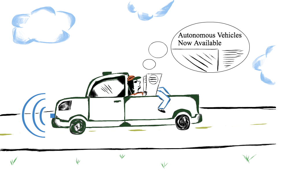
Between levels 2 and 3, there is an important shift in the classification system. This is where the primary controller of the vehicle, responsible for most DDTs, shifts from the human driver to the autonomous vehicle system. To date, some self-driving cars have achieved SAE level 4, but none have reached the complete autonomy of level 5.
 A cartoon illustration depicting a level 5 driving experience.
Before a completely automated driving experience can become reality, there are still roadblocks to address. One important design challenge in the field of autonomous driving is the optimization of light detection and ranging (lidar) systems. Lidar works similarly to sonar and radar but relies on light instead of sound or radio waves. Its use enables self-driving cars and other autonomous robots to have a three-dimensional perception of their surroundings. Lidar also has many applications in industries where surveying of terrain is needed, such as archaeology and forestry.
How Lidar Works
The working principle of lidar is deceptively simple: send an intense, narrow beam of light in a specific direction; measure how long it takes backscattered light to reach a receiver placed in close proximity to the light source (known as the time of flight); and from the time of flight, calculate the distance to the scattering surface. Repeat the process for a range of beam angles and compile the data. The result is an image of your surroundings — except that each pixel quantifies depth, not color, as in a typical image.
Here we only need one simple formula to convert the time of flight t to distance d. Assuming that the light propagates in a medium of constant refractive index n, we have:
where c_0 is the speed of light in a vacuum. In the applications below, we consider lidar in air, so we set n=1.
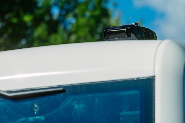 An example of a lidar unit attached to the roof of a vehicle. Image by Arno Mikkor — Own work. Licensed under CC BY 2.0, via Flickr Creative Commons.
There are, however, a number of practical considerations required for a functional lidar system:
- A pulsed laser is an obvious choice of light source to allow rapid scanning with a tight beam, but attention must be paid to eye safety; wavelengths of around 1550 nm are usually preferred since they carry no risk of eye damage even with direct exposure.
- To facilitate accurate scanning, the beam angle must be precisely controllable. This can be achieved by using MEMS mirrors, for example.
- Eye-safe light with a longer wavelength can be tricky to detect efficiently due to the low energy of the photons. A common choice is a preamplified avalanche or PIN photodiode.
Fundamentally, lidar works in a similar way to radar and sonar, but compared to these older technologies, lidar offers a few key advantages. For example, the wavelength of light used by lidar (usually around 1550 nm) is much shorter than that of the radio waves used by radar or the sound waves of sonar, making its resolution superior. Additionally, sound waves are attenuated by air much more strongly than light, so lidar has a longer range. Sonar is generally used only underwater, where the attenuation is much weaker. Lastly, the speed of light in air is much less sensitive to variations in temperature and pressure than that of sound, so distances obtained with lidar are more accurate than sonar.
Lidar also has some limitations to consider. Unlike radar and sonar, lidar cannot exploit the Doppler effect to obtain information about the speed of objects, so a sufficiently high refresh rate is needed to allow inference of speeds by rate of change of distance. Also, transparent and mirror-like surfaces do not backscatter much light, making them difficult to detect by lidar.
Modeling Lidar with the Ray Optics Module
The time domain ray-tracing algorithm in COMSOL Multiphysics® is ideally suited for lidar modeling. Compared to the conventional geometrical ray-tracing methods, more accurate lidar simulation is possible with access to the actual arrival time of each ray. This is illustrated in the figure below. For details about the Ray Optics Module, check out this blog post. Let’s take a look at two example models of lidar: a car detecting obstacles at an intersection and a robot vacuum cleaner mapping out a room layout. In both models, lidar units are implemented simply as pairs of release features (light sources) and accumulators (detectors).
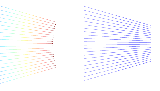 Illustration of the difference between time-dependent ray tracing in COMSOL Multiphysics® (left) and standard sequential plane-to-plane ray tracing (right).
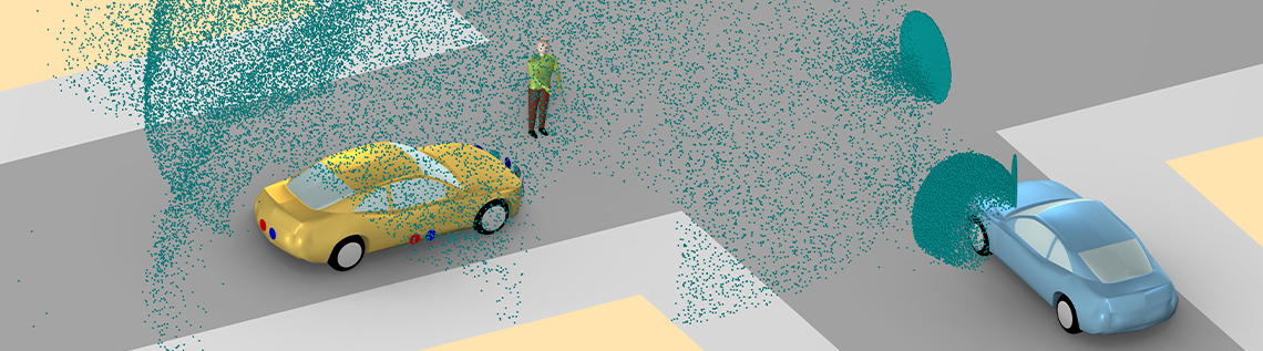
Detecting Obstacles with Lidar
This model consists of a car equipped with lidar units detecting a pedestrian and another car at an intersection. An animation of the ray trace and a plot of the time-dependent signal at the three front detectors are shown below. It should be noted that only a single detection cycle is considered here, and in reality, this process is repeated several times per second.
Animation of the ray-tracing results for the car lidar model.
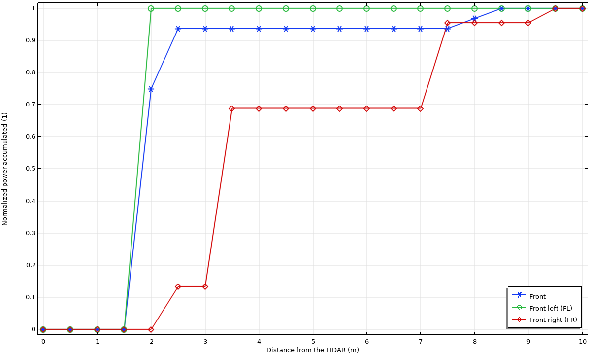 Plot showing the signal detected at the three front detectors. The front and front-left detectors peak at 2 m, detecting the pedestrian. The front-right detector peaks at 7.5 m, detecting the other car.
Scanning a Room with Lidar
Our second example model shows a robot vacuum cleaner scanning a room with a rotating lidar unit. We see in the figure below that the room layout can be recovered from a plot of the time of flight against rotation angle.
An animation of the lidar angle sweep showing the ray trajectories.
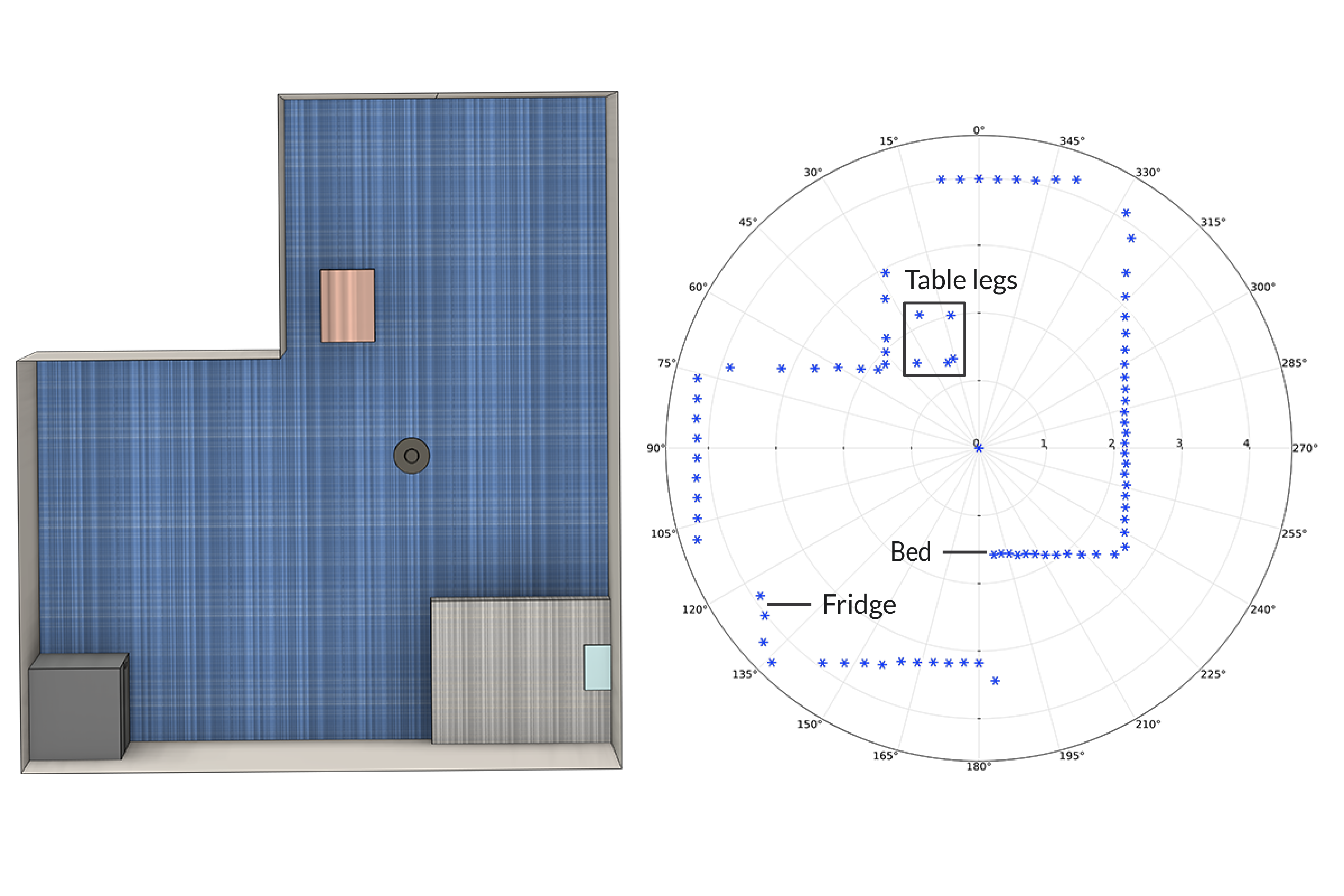
A comparison between the room layout (left) and the time of flight (distance) as a function of the angle of the lidar unit (right).
Next Steps
Try modeling a lidar system yourself. From the Application Gallery, you can download the model files for the examples featured here:


Comments (0)