How to Implement the Fourier Transformation from Computed Solutions

We previously learned how to calculate the Fourier transform of a rectangular aperture in a Fraunhofer diffraction model in the COMSOL Multiphysics® software. In that example, the aperture was given as an analytical function. The procedure is a bit different if the source data for the Fourier transformation is a computed solution. In this blog post, we will learn how to implement the Fourier transformation for computed solutions with an electromagnetic simulation of a Fresnel lens.

Fourier Transformation with Fourier Optics

Implementing the Fourier transformation in a simulation can be useful in Fourier optics, signal processing (for use in frequency pattern extraction), and noise reduction and filtering via image processing. In Fourier optics, the Fresnel approximation is one of the approximation methods used for calculating the field near the diffracting aperture. Suppose a diffracting aperture is located in the (x,y) plane at z=0. The diffracted electric field in the (u,v) plane at the distance z=f from the diffracting aperture is calculated as

where, \lambda is the wavelength and E(x,y,0), \ E(u,v,f) account for the electric field at the (x,y) plane and the (u,v) plane, respectively. (See Ref. 1 for more details.)

In this approximation formula, the diffracted field is calculated by Fourier transforming the incident field multiplied by the quadratic phase function {\rm exp}\{-i\pi (x^2+y^2)/(\lambda f)\}.

The sign convention of the phase function must follow the sign convention of the time dependence of the fields. In COMSOL Multiphysics, the time dependence of the electromagnetic fields is of the form {\rm exp}(+i\omega t). So, the sign of the quadratic phase function is negative.

Fresnel Lenses

Now, let’s take a look at an example of a Fresnel lens. A Fresnel lens is a regular plano-convex lens except for its curved surface, which is folded toward the flat side at every multiple of m \lambda/(n-1) along the lens height, where m is an integer and n is the refractive index of the lens material. This is called an m^th-order Fresnel lens.

The shift of the surface by this particular height along the light propagation direction only changes the phase of the light by 2m \pi (roughly speaking and under the paraxial approximation). Because of this, the folded lens fundamentally reproduces the same wavefront in the far field and behaves like the original unfolded lens. The main difference is the diffraction effect. Regular lenses basically don’t show any diffraction (if there is no vignetting by a hard aperture), while Fresnel lenses always show small diffraction patterns around the main spot due to the surface discontinuities and internal reflections.

When a Fresnel lens is designed digitally, the lens surface is made up of discrete layers, giving it a staircase-like appearance. This is called a multilevel Fresnel lens. Due to the flat part of the steps, the diffraction pattern of a multilevel Fresnel lens typically includes a zeroth-order background in addition to the higher-order diffraction.

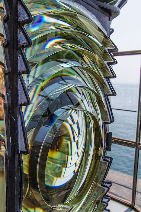
A Fresnel lens in a lighthouse in Boston. Image by Manfred Schmidt — Own work. Licensed under CC BY-SA 4.0, via Wikimedia Commons.

Why are we using a Fresnel lens as our example? The reason is similar to why lighthouses use Fresnel lenses in their operations. A Fresnel lens is folded into m \lambda/(n-1) in height. It can be extremely thin and therefore of less weight and volume, which is beneficial for the optics of lighthouses compared to a large, heavy, and thick lens of the conventional refractive type. Likewise, for our purposes, Fresnel lenses can be easier to simulate in COMSOL Multiphysics and the add-on Wave Optics Module because the number of elements are manageable.

Modeling a Focusing Fresnel Lens in COMSOL Multiphysics®

The figure below depicts the optics layout that we are trying to simulate to demonstrate how we can implement the Fourier transformation, applied to a computed solution solved for by the Wave Optics, Frequency Domain interface.

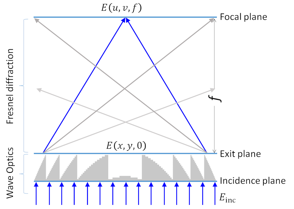
Focusing 16-level Fresnel lens model.

This is a first-order Fresnel lens with surfaces that are digitized in 16 levels. A plane wave E_{\rm inc} is incident on the incidence plane. At the exit plane at z=0, the field is diffracted by the Fresnel lens to be E(x,y,0). This process can be easily modeled and simulated by the Wave Optics, Frequency Domain interface. Then, we calculate the field E(u,v,f) at the focal plane at z=f by applying the Fourier transformation in the Fresnel approximation, as described above.

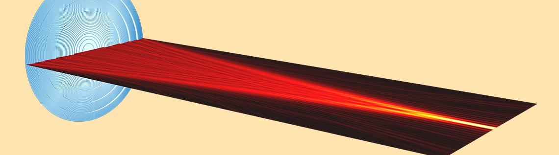
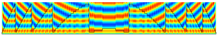
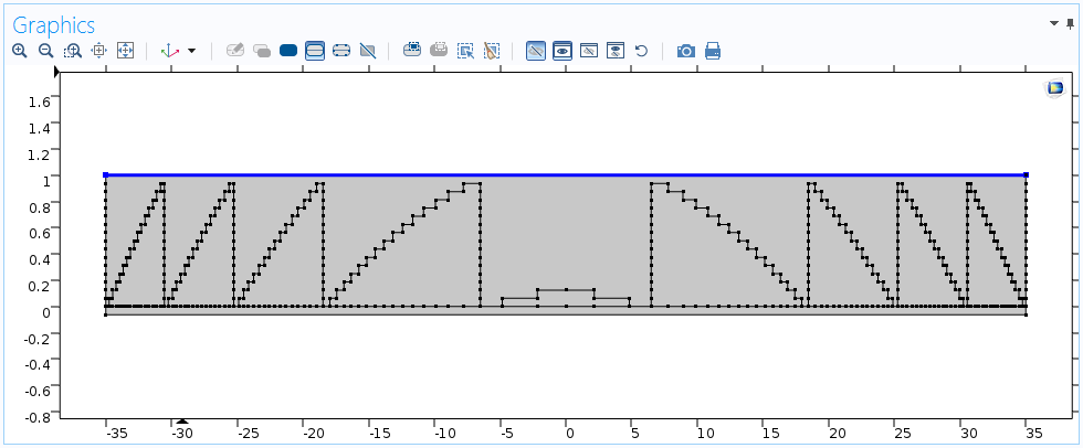
The figures below are the result of our computation, with the electric field component in the domains (top) and on the boundary corresponding to the exit plane (bottom). Note that the geometry is not drawn to scale in the vertical axis. We can clearly see the positively curved wavefront from the center and from every air gap between the saw teeth. Note that the reflection from the lens surfaces leads to some small interferences in the domain field result and ripples in the boundary field result. This is because there is no antireflective coating modeled here.

The computed electric field component in the Fresnel lens and surrounding air domains (vertical axis is not to scale).

The computed electric field component at the exit plane.

Implementing the Fourier Transformation from a Computed Solution

Let’s move on to the Fourier transformation. In the previous example of an analytical function, we prepared two data sets: one for the source space and one for the Fourier space. The parameter names that were defined in the Settings window of the data set were the spatial coordinates (x,y) in the source plane and the spatial coordinates (u,v) in the image plane.

In today’s example, the source space is already created in the computed data set, Study 1/Solution 1 (sol1){dset1}, with the computed solutions. All we need to do is create a one-dimensional data set, Grid1D {grid1}, with parameters for the Fourier space; i.e., the spatial coordinate u in the focal plane. We then relate it to the source data set, as seen in the figure below. Then, we define an integration operator intop1 on the exit plane.

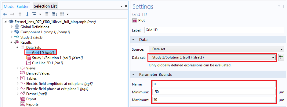
Settings for the data set for the transformation.

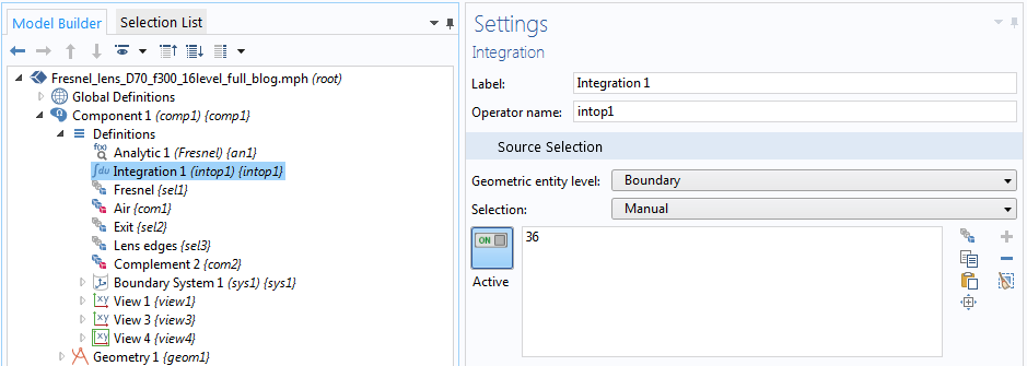
The intop1 operator defined on the exit plane (vertical axis is not to scale).

Finally, we define the Fourier transformation in a 1D plot, shown below. It’s important to specify the data set we previously created for the transformation and to let COMSOL Multiphysics know that u is the destination independent variable by using the dest operator.

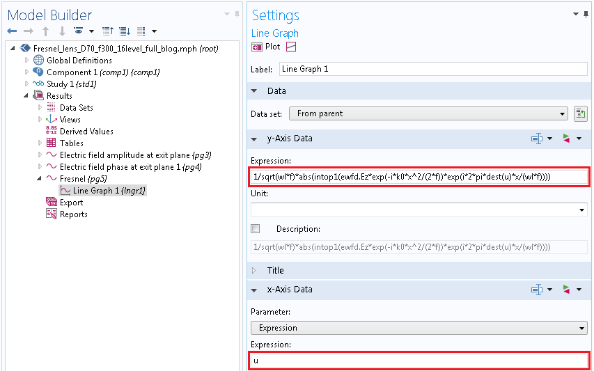
Settings for the Fourier transformation in a 1D plot.

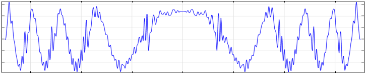
The end result is shown in the following plot. This is a typical image of the focused beam through a multilevel Fresnel lens in the focal plane (see Ref. 2). There is the main spot by the first-order diffraction in the center and a weaker background caused by the zeroth-order (nondiffracted) and higher-order diffractions.

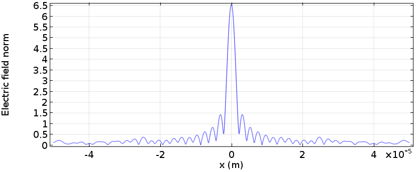
Electric field norm plot of the focused beam through a 16-level Fresnel lens.

Concluding Remarks

In this blog post, we learned how to implement the Fourier transformation for computed solutions. This functionality is useful for long-distance propagation calculation in COMSOL Multiphysics and extends electromagnetic simulation to Fourier optics.

Next Steps

Download the model files for the Fresnel lens example by clicking the button below.

Read More About Simulating Wave Optics

• Simulating Holographic Data Storage in COMSOL Multiphysics
• How to Simulate a Holographic Page Data Storage System
• How to Implement the Fourier Transformation in COMSOL Multiphysics

References

1. J.W. Goodman, Introduction to Fourier Optics, The McGraw Hill Company, Inc.
2. D. C. O’Shea, Diffractive Optics, SPIE Press.