
There are a few things that I learned in my university electrical engineering classes that I really wish would have been taught a bit differently. The concepts of voltage and ground fall into this category, as these terms are often misused in subtle ways. We will give them a precise definition and talk about some interesting cases from the point of view of understanding electromagnetics and building good computational models.
A Textbook Example
Let’s start by thinking of one of the original and simplest electrical devices: the battery. In its simplest form, a battery can be made by sticking two pieces of metal into an orange. We can use a battery in an electrical device, such as a flashlight. One of the first things we learned in our electrical engineering classes was how to draw a circuit diagram, which probably looked a little bit like the following:
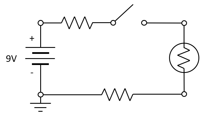
An elementary circuit diagram of a flashlight.
This figure shows that we have a battery with one terminal connected to a switch. Once the switch is closed, current will flow through the bulb (emitting light) and through the resistors back to the other battery terminal. This device is operating at DC (time-invariant) conditions. The resistors represent the internal resistance of the battery as well as of the connecting wires. The points connecting these components are referred to as the nodes of the circuit.
An exercise we were most likely given in school was to compute the current through the circuit, as well as the voltages at the various nodes. But what exactly is voltage, in this context? Voltage is defined as the difference in the electric potential between two nodes in the circuit, such as the two nodes of the battery. However, note that we also drew a ground at one terminal of the battery, and we were also given the definition of ground as: the node where the electric potential is zero. So, if we are given a 9 Volt battery, we now know the electric potential of the other battery terminal, and we can use Kirchoff’s laws to figure out all of the other node voltages relative to the ground node, as well as the current.
This should raise a question, though: Why do we call that particular node ground? The circuit we have here represents a flashlight, and a flashlight will still work if it’s entirely electrically isolated from anything else. (You can verify that by tossing a flashlight into the air.) What exactly is this point in our network that we call ground? It is a completely arbitrary, but very numerically convenient, definition. We could actually have chosen any other point in the circuit as ground (or even assigned a value different from zero) and gotten the exact same solution for the current. The node voltages would just be different by a constant. That is, if we have a solution for the electric potentials of the nodes, \mathbf{V} = \{V_1, V_2, V_3, V_4\}, we can theoretically add any constant \mathbf{V} = \{V_1+c, V_2+c, V_3+c, V_4+c\} and still have a valid solution.
There is a caveat to this, however. We are solving this problem on a computer, and computers work in finite precision arithmetic, so we wouldn’t want to add an outrageously large constant, such as 10^{16} \approx 1/\epsilon, where \epsilon is double precision floating point relative accuracy, since this would start to introduce numerical issues. Setting one arbitrary node in the model to zero (to ground) is thus not just pedagogically convenient, it is also good numerical modeling practice.
When solving for the electric currents within a set of domains using the finite element method, not much changes. The finite element method can be thought of as a spatially distributed form of Kirchoff’s law. That is, a finite element model is essentially just a much more complicated circuit diagram, and to numerically solve it, we just need to set an arbitrary point in the modeling space to ground.
Hold On! Do You Mean Ground Is Arbitrary and Just There for Numerical Purposes?
I can already hear a few power engineers grinding their teeth, as the term ground most certainly also has a very real physical meaning. We also define ground as Earth, that big ball of matter below our feet that we connect grounding straps to. We know exactly what it is; it’s a very physical thing. But what does it mean from an electrical modeling point of view?
Electrically speaking, Earth is a very large mass of conductive material, and (at least for the purposes of this discussion) has a relatively negligible resistance. This leads to a second definition of ground: It is domain that is touching our model and is assumed to have relatively negligible variation in electric potential when current flows through it, as compared to the potential distribution within our model.
This new definition is clearly distinct from the previous one, and sometimes people call this “Earth ground”. There is also the analogous concept of “chassis ground” or “frame ground” (think of an airplane flying in the sky or the chassis of your car), but even just a really big busbar running through a factory can also be defined as a ground.
The big difference here is we’ve changed our definition of ground from just a single point to a volume of space. This volume of space represents an infinite source, and sink, for current. That is, electrons can flow in or out of this ground domain forever, as long as there exists a potential difference relative to ground due to a battery or generator.
For computational modeling purposes, we don’t even need to model this ground domain at all; we just need to specify the boundary where our modeling domain touches this domain. Since we’ve already said that we will assume negligible electric variation within this domain, we can justify applying a uniform electric potential over this entire surface, and for the numerical reasons described earlier, we choose an electric potential of zero. We have now arrived at the definition of ground that we can use for modeling of DC electrical systems: A boundary of zero electric potential that represents a domain that is an infinite source, or sink, for current.
Next, we will look at how these definitions affect our modeling approach.
Modeling Voltage and Ground in COMSOL Multiphysics®
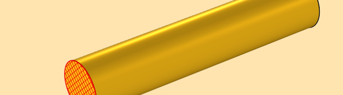
Consider just a straight section of circular wire. We will assume that one end is connected to ground and the other end connected to a source.
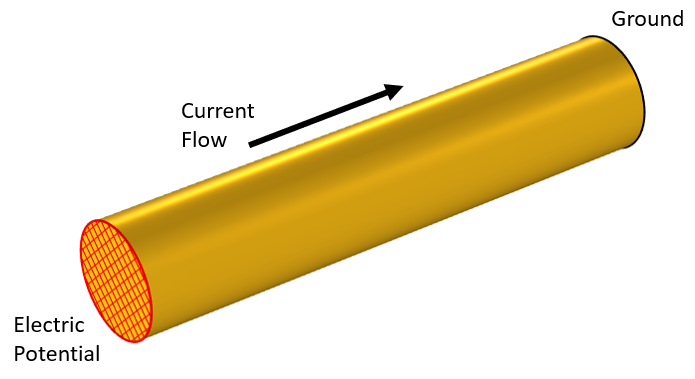
A model of a section of current-carrying wire.
When solving for current flow under DC conditions, we use a combination of these boundary conditions within the Electric Currents interface:
- The Ground condition
- The Electric Potential condition
- The Normal Current Density condition
- The Terminal condition (only available with the AC/DC Module, MEMS Module, Semiconductor Module, or Plasma Module)
The Ground and Electric Potential are nearly the same condition. They fix the electric potential across and entire surface. The Ground condition simply fixes the electric potential to exactly zero, while you can enter different values via the Electric Potential condition. Keep in mind the previous definition: These boundaries represent the boundary to a domain that is an infinite sink (or source) of current, and any electric potential difference within that domain is negligible relative to our modeling domain. If you’re modeling the wires connected to the terminals of a battery, these are appropriate boundary conditions to use.
The third option, Normal Current Density, specifies the current flux into the model through a surface. It does not fix the electric potential to be uniform across the boundary. A model with a Normal Current Density condition typically also has a Ground condition, through which all of the injected current leaves.
One can also have a well-posed finite element model that has two Normal Current Density features, one that injects current and one that removes current. As long as the sum of these currents is exactly zero, there exists a solution. To find this solution, it is good practice to add a Point Ground condition to any arbitrary point for the reasons discussed earlier. But, interestingly, when modeling in 3D, we can actually omit the Point Ground condition entirely and just have two Normal Current Density features, as long as they inject and remove exactly the same amount of current on the given finite element mesh. The resulting problem will be ungauged, but in 3D models, we use an iterative solver, which will “pick its own gauge” and still converge, even though the electric potential field is underconstrained. For more details on gauge fixing, see the previous blog posts “What Is Gauge Fixing: A Theoretical Introduction” and “How Do I Use Gauge Fixing in COMSOL Multiphysics®?“. This point, though, is more of a mathematical curiosity for the very interested reader.
Lastly, the Terminal condition is worth mentioning separately. The terminal condition has the option of specifying the electric potential, in which case it is functionally identical to the Electric Potential condition. It also has the option of specifying the total current. When the current is specified, the Terminal condition applies an additional equation that solves for the electric potential over the surface such that the desired total current flows in or out of the model. The Terminal condition additionally automatically computes resistances and other quantities of interest, so if you have either the AC/DC Module or the MEMS Module, it is generally the preferred option. There are also other options within the Terminal condition to specify a circuit connection or to specify the dissipated power, or to specify a terminated connection to a transmission line, for S-parameter computations. These more advanced conditions are covered in our lecture series on modeling considerations for resistive and capacitive devices.
Once you have solved your model, you’ll also want to extract data from it. Via the finite element method, the software computes the field V(\mathbf{x}), and from this, we can extract the electric field, \mathbf{E} = – \nabla V, and current, \mathbf{J} = \sigma \mathbf{E}, as well as the magnitude (the norm) of any of these vector fields. Keep in mind that these fields will be convergent with mesh refinement, except in the locality of any singularities in the model, which you may, or may not, want to address.
Finally, note that you can take the line integral of the electric field between two points in the model, and this integral will equal the difference in the electric potential between these two points. Since we are dealing with a scalar potential field, this integral is path independent:
The above equation, which defines the voltage as the path integral of the electric field, is not always true once we move to modeling of time-varying electromagnetic fields. That is a topic for another blog post, so stay tuned!
Further Reading
- Read the follow-up to this blog post: “Voltage and Ground When Modeling Wave-Like EM Fields“
- Check out this related Learning Center article here: “Modeling TEM and Quasi-TEM Transmission Lines“


Comments (1)
Ivar KJELBERG
July 17, 2021Hi Walter,
Thanks for great Blog posts and all your videos the last year, you know you should be regularly references by the professors, for all physics students, these Blogs are really nice illustrated explanations helping students to understand the basics of Physics 🙂
Have fun COMSOLing
Ivar