Minimizing the Charging Time of a Battery

Batteries are used for many different kinds of portable electronic products, and the relative importance of various performance criteria depends on the application. However, charging time and longevity are often important because they both relate to time and, therefore, also economics. In this post, we will investigate the relationship between these two performance criteria for a lithium-ion battery using the capabilities of the Optimization Module, an add-on product to the COMSOL Multiphysics^® software.

Lithium-Ion Batteries

Let’s consider a 1D model of a lithium jelly roll consisting of graphite for the negative electrode, NMC 111 for the positive electrode, and 1.0 M LiPF₆ for the electrolyte. The degradation is calculated based on a generalized volumetric Butler–Volmer expression in the negative graphite electrode current:

where c_l is the electrolyte salt concentration, while \phi_s and \phi_l are the electric and electrolyte potentials, respectively. The charge loss can then be computed by integrating over the negative electrode 

and this is a good measure of the battery degradation during a charge cycle. We then compute the number of cycles resulting in a 10% degradation and constrain this variable based on the maximum number of allowed cycles.

Time-Optimal Control

The purpose of the optimization is to minimize the charging time while constraining the degradation charge. This is achieved by changing the charging profile. A Control Function feature is used to allow the charging current to vary with time. The problem can be regularized in different ways, and here we use a function based on five second-order Bernstein polynomials where the shared points are taken as the average of the midpoints so that the slope of the function becomes continuous. The time-dependent solver must stop when the battery is full, so the stop condition is set based on the integral of the control function.

The animation below illustrates how the progress of an optimization might look like for a battery designed to last 2000 charging cycles.

The MMA (method of moving asymptotes) optimization solver reduces the charging time without violating the constraint on the degradation charge. Note that the number of optimization iterations has been artificially increased using a move limit for visualization purposes.

The Pareto optimal front of the charging time versus the degradation can be traced by varying the degradation charge.

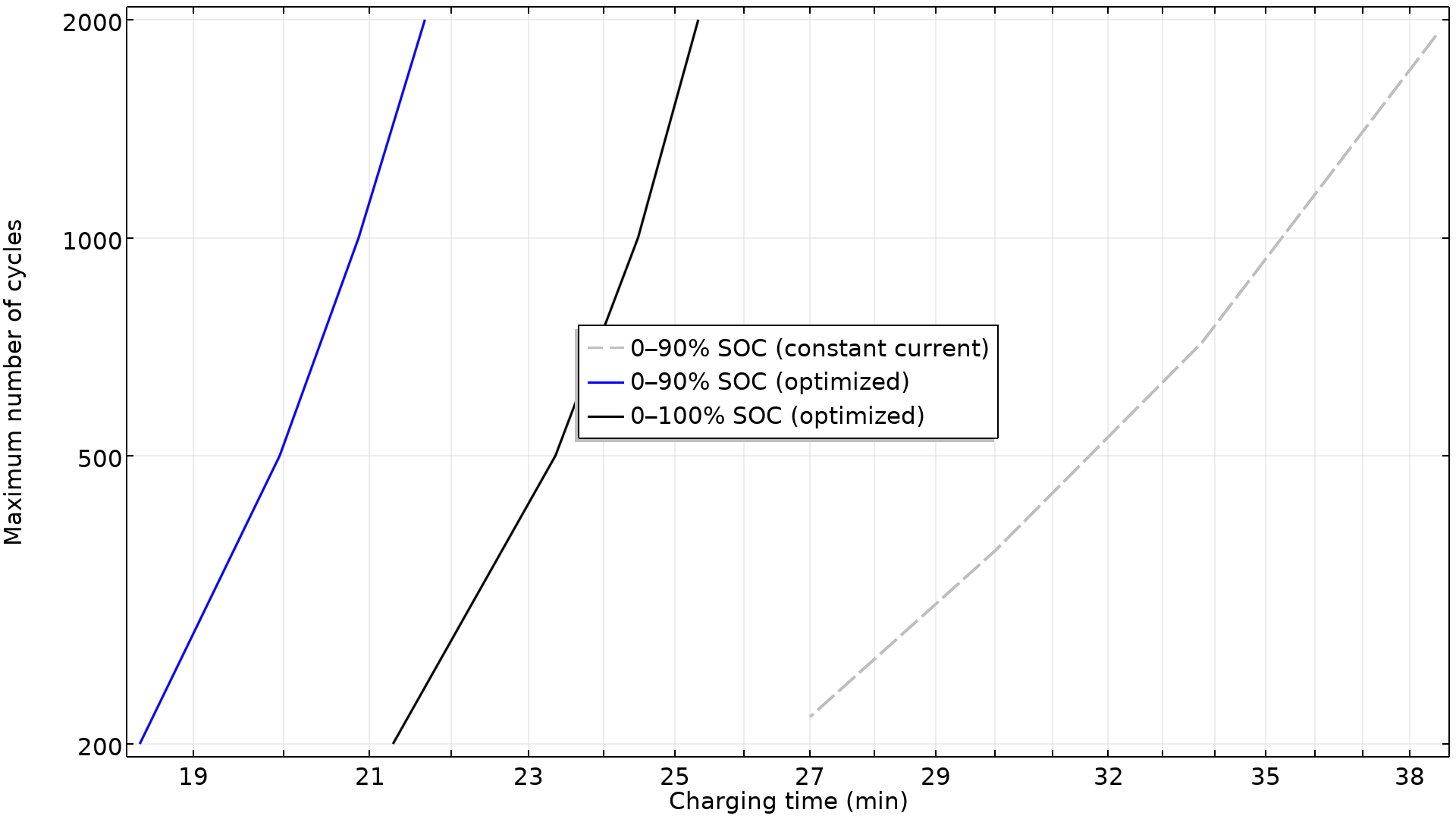The maximum number of cycles is plotted versus the charging time for charging to 90% and 100% state of charge (SOC). The result of a constant charging current (dashed line) is also included to better illustrate the benefit of a time-varying current.

The degradation charge has an exponential dependence on the charging time; a ~4-minute-longer charging time increases the maximum number of cycles by a factor of 10. The result of using a constant current is included for reference, and this shows that it takes 38 minutes to charge the battery 90% with a constant current, while it only takes 22 minutes with an optimized charging profile. Finally, one can get down to 18 minutes if the battery only has to last 200 cycles.

Takeaways

The degradation of a battery is highly sensitive to the charging rate, so significant improvements in battery longevity can be gained with modest sacrifices in the charging time. The functionality for gradient-based optimization with a condition-based final time can be used for a wide range of optimal control problems, including time-optimal control.

Next Steps

• Interested in the details of this model’s setup in COMSOL^®?
  • Download and explore it for yourself: Minimizing the Charging Time of a Lithium-Ion Battery
• Want to learn more about optimization?
  • Check out these previous blog posts.