Optimization of Heat Exchangers

When designing heat exchangers, it’s essential to consider the heat transfer rate, hydraulic resistance, and efficiency, and for some applications, it’s also important to consider the structural integrity. However, spending time and resources to study these components will be in vain if there is no affordable way to manufacture the finished product. Considering costs of design and manufacturing throughout the design process makes the development of heat exchangers a difficult task. Here, we will explore the possibility of using shape and topology optimization to tackle such design challenges.

Shape Optimization

Shape optimization works the same way regardless of the physics, and that makes it simpler to use than topology optimization. However, it should be noted that shape and topology optimization both involve many design variables, so gradient-based optimization is required in any case. Gradient-based optimization is significantly faster than derivative-free methods, when many design variables are involved, because it efficiently uses sensitivity information to guide each iteration instead of relying on costly sampling or brute-force searches. The examples shown here rely on the method of moving asymptotes (MMA) optimization algorithm and automatic gradient computation.

First, we’ll focus on shape optimization of a plate heat exchanger, and then we’ll consider the sizing of pipes in a shell-and-tube heat exchanger.

Readers interested in a more general introduction to shape optimization should check out our blog post “Shape Optimization in Electromagnetics: Part 1”.

The hydraulic resistance of a heat exchanger can be limited by imposing a constraint on the pressure drop for a given imposed flow rate, but the optimization will tend to make a design corresponding to the maximum allowed value for the pressure drop, so in practice the applied pumping power and hydraulic resistance will be fixed. Alternatively, one can impose a pressure-driven flow and let the optimization choose the pumping power and hydraulic resistance. This method is computationally cheaper, and we will therefore focus on this option.

We’ll first consider a plate heat exchanger in the laminar flow regime, where the heat transfer rate is maximized by allowing the shape of the plate to change, as illustrated in the animation below. The optimization improves the heat exchange by 30% relative to the initial design with a flat plate.

The optimized plate heat exchanger forces the flow around the corners of the volume, as illustrated by the streamlines colored by the temperature. Note that the deformation is exaggerated by a factor of two in the gray surface representation of the design.

Let’s now look at the second example, a shell-and-tube heat exchanger in the turbulent flow regime. Again, we maximize the heat transfer rate, but this time we allow the size and position of the tubes to change. In this case, the optimization is only able to improve the heat exchange rate by 5%, which might be due to less design freedom relative to the previous example.

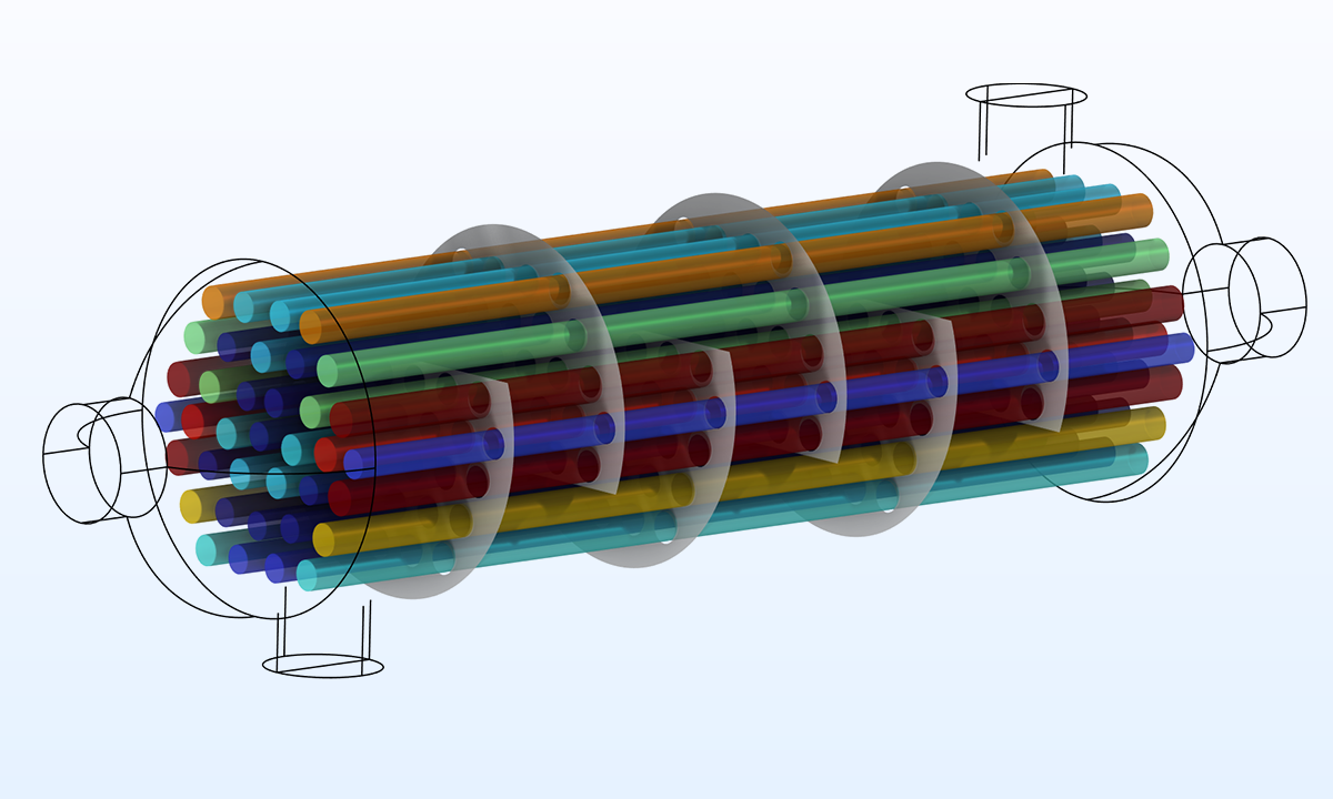The optimized shell-and-tube heat exchanger is illustrated with the tubes colored by their diameter. The smaller tubes near the center reduce the variation of the flow rate from tube to tube.

Topology Optimization

Topology optimization with the density method works by assigning a design variable to every computational element. In the case of structural mechanics, zero corresponds to void, while one corresponds to solid.

Readers interested in a more detailed introduction to topology optimization should check out our blog post “Performing Topology Optimization with the Density Method”.

For the topology optimization of heat exchangers, the task is to identify which region should belong to which fluid, so typically a design variable equal to zero corresponds to one fluid, while the other fluid corresponds to one (Ref. 1). This strategy avoids mixing of the two fluids as long as there is no grayscale in the final design, i.e., the design variables are equal to zero or one but not intermediate values. The strategy can be extended to account for the solid domain between the fluids, but we will omit this here. The no-slip boundary condition is enforced with a Darcy penalization term, a strategy similar to other applications of fluid topology optimization:

where \mathbf{u}_\mathrm{cold} and \mathbf{u}_\mathrm{hot} are the flow velocity for the hot and cold domains, which are solved using separate PDEs. \alpha_\mathrm{max} is the maximum damping, which dampens the flow so that both flow velocities cannot be large at the same time. q determines the damping for intermediate values of the design variable field, \theta, and low values tend to be associated with grayscale designs being optimal, while larger values generate more discrete, clearly separated regions, leading to designs that are physically realizable.

Energy conservation is handled using a convection-diffusion equation for the temperature, where the convective term depends on the total velocity field, given by the sum \mathbf{u}_\text{hot} + \mathbf{u}_\text{cold}. Although this sum does not explicitly depend on the design variables, in practice, each velocity field dominates in its respective fluid region, so the flow speeds are only comparable in the transition zone between the fluids.

Heat exchangers generally operate in the turbulent regime, but the topology optimization results shown here are limited to the laminar flow regime because turbulence models require resolution of boundary layers, and that is extremely expensive for the uniform meshes used with topology optimization.

Large channels give low hydraulic resistance, while small channels provide good heat exchange. The optimal heat exchanger topology is thus expected to consist of intermingled pipes that branch into thin pipes in a small area where the actual heat exchange occurs, but this is not possible in two dimensions since the mixing constraint effectively fixes the topology.

Two twisted and parallel tubes are produced when maximizing the heat exchange between two fluids using topology optimization in two dimensions.

It is computationally expensive to perform topology optimization in 3D, so in this final example model mirror symmetry is imposed to reduce the design domain by a factor of two. Furthermore, rotational symmetry is imposed on the flow so that only the flow of one of the fluids needs to be computed. Finally, the objective considers both the heat transfer rate and the hydraulic dissipation. Both should be maximized, because maximizing the hydraulic dissipation for a pressure-driven flow will minimize the hydraulic resistance. The objectives can be combined with a maximin formulation, but that is computationally expensive, so a p-norm is used instead:

where \kappa is a weight that controls the relative importance of the objectives, and P controls the accuracy of the approximation. The results shown here do not consider the efficiency in the objective because it prevents discrete designs, but you can use it initially so as to nudge the design toward minima with better efficiency. 

The raw design variable field is animated on five slices to illustrate how the optimal design becomes more discrete as q is increased.

The optimized result is smoothed so that the design can be verified with an explicit geometry representation. This can be seen in the animation below. The camera is fixed, but the design is somewhat transparent, so it is possible to see what goes on inside the structure. Alternatively, one can explore the interactive model file below where the design is fixed, where the camera can be manipulated. Only half of the design is shown, as this makes it easier to see the internal intricacies of the design.

The optimized heat exchanger consists of two domains that branch into each other to allow strong thermal coupling in small tubes without introducing excessive hydraulic resistance.

Overview of Optimization Functionality

This blog post has focused on heat exchangers with stationary flow, but the underlying functionality is flexible in the sense that problems involving other physics can also be solved with gradient-based optimization. It is even possible to combine different physics and still have the gradient be computed automatically for custom objectives and constraints. The shape and topology optimization interfaces can be used to set up the design variables, and probes simplify the setup of constraints and objectives. However, constraints and objectives are highly application-specific, so this part of the modeling process can require some experimentation. Finally, it is possible to perform gradient-based optimization considering eigenfrequencies or transient problems.

Readers interested in examples involving eigenfrequency optimization should check out our blog post “Maximizing Eigenfrequencies with Shape and Topology Optimization”.

Webinar on the Optimization of Thermal Management Systems

To learn more about how optimization can be used to automatically generate high-performance designs for heat exchangers and fluid flow systems, attend our upcoming webinar on the optimization of thermal management systems. The webinar will be held on Wednesday, September 3, at 15–15:45 CEST.

Reference

1. P. Papazoglou, Topology Optimization of Heat Exchangers, master’s thesis, Delft University of Technology, 2015.