Understanding Classical Gray Body Radiation Theory

Even though the first man-made light source used thermal radiation, the effect wasn’t fully understood until the discovery of quantum mechanics. Nowadays, it’s a well-known physics concept. In this blog post, we discuss surface-to-surface radiation theory for the so-called gray body, how to implement it in the COMSOL Multiphysics® software, and an interesting use of this theory.

Classical Thermal Radiation Theory

Candlelight was the first man-made light source. Much later, gas lights emerged. Then, in the 19^th century, the first electric incandescent lamp was invented. 140 years later, the incandescent lamp is being replaced by the LED.

Candles, gas lights, and incandescent lamps all use thermal radiation, the only heat transfer phenomenon that works without the presence of heat-conductive media. Without this special property, we wouldn’t be able to live on Earth: Solar energy would pour in by this mechanism through a vacuum.

An incandescent light bulb.

One of the most interesting stories in physics is when Max Planck discovered the formula of the spectral distribution, now called the Planck distribution, for black body radiation. The black body is an idealized physical body that absorbs all incident electromagnetic radiation; equivalently, a body that emits maximized thermal radiation.

The discovery of the black body theory opened the door to quantum mechanics. With Planck’s work, we now know how much power we get from a black body object at temperature T in an equilibrium state, which is called the Stefan-Boltzmann law:

where \sigma \simeq 5.67 \times 10^{-8} \; \; \; (W/m^2 \cdot K^4) is the Stefan-Boltzmann constant and n is the refractive index of the media.

We now consider more practical objects, called gray bodies. A gray body is an imperfect black body; i.e., a physical object that partially absorbs incident electromagnetic radiation. The ratio of a gray body’s thermal radiation to a black body’s thermal radiation at the same temperature is called the emissivity of the gray body.

The emissivity of a black body is unity, while that of a gray body is larger than 0 and smaller than 1. The emissivity is a function of the geometry of the radiative surface, its physical properties, and the wavelength. So, how is emissivity determined from certain structures?

For the sake of simplicity, we will consider the diffuse gray surface, which doesn’t account for the spectral dependency of the radiation, throughout this section. The following theory is based on Gouffé’s paper (Ref. 1), which outlines the classical gray body radiation theory. The math is something that you might have learned in middle or high school, but the physical concept is a little more complicated. Gouffé’s paper was cited by many researchers at the time it was published (Ref. 7). In this blog post, we will try to include what is missing from the original paper in order to provide a complete explanation.

First of all, let’s define our terms and conventions. When we mention reflectivity and absorptivity in this blog post, we must differentiate between the “material” and “apparent” quantities. This is very important in order to avoid confusion when learning about thermal radiation. Because gray bodies typically have certain (tiny) structures on their surfaces, the “apparent” quantity viewed from a far field is different from the raw material quantity. For example, the apparent reflectivity of a rough surface is always lower than its material reflectivity.

Our goal is to calculate the apparent emissivity from a given material reflectivity and the geometry of the structure. Here, we will differentiate “material” quantities from “apparent” quantities by appending “_0” in the notation. Otherwise, it is understood that we are talking about a quantity in general. The nomenclature of the terms is as follows:

• Material reflectivity, \rho_0
• Material absorptivity, \alpha_0
• Material emissivity, \varepsilon_0
• Apparent reflectivity, \rho
• Apparent absorptivity, \alpha
• Apparent emissivity, \varepsilon
• Cavity’s internal area, S
• Opening area, A
• View angle, \theta
• View factor (normalized solid angle), F
• View factor (area ratio), G

From the conservation law of energy, we have the following relation for opaque materials between the reflectivity \rho and the absorptivity \alpha:

Kirchhoff’s law states that the material emissivity \varepsilon at thermodynamic equilibrium is equal to the absorptivity \alpha; i.e.,

From the two relations above, we get the emissivity from the reflectivity; i.e.,

We consider a single surface structure, as shown in the following figure. The structure can be anything, but in this blog post, we use a spherical cavity with an opening on top with area A (circle of radius R) at distance L from the bottom of the cavity. We assume that the material reflectivity \rho_0 is uniform over the internal surface of the cavity and the reflection takes place according to Lambert’s law; i.e., the intensity of the reflection is I_r = \rho_0 \cos \theta, where \theta is the viewing angle, as depicted in the figure. We want to calculate how much apparent reflection we get out of an incident light of the energy of unity.

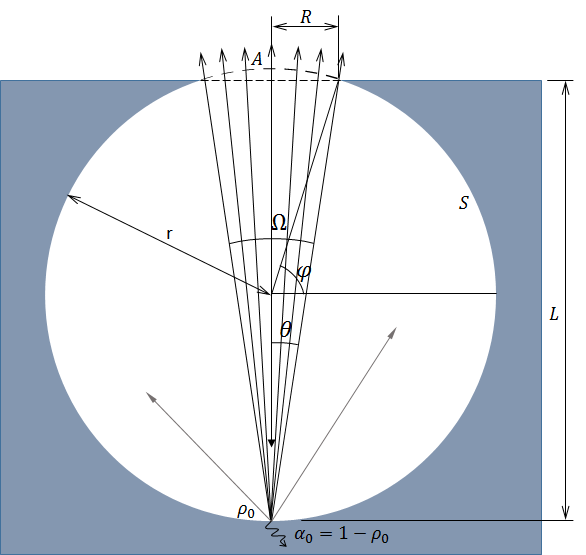
Surface structure for calculating the apparent reflectivity.

As the first-order approximation, the reflection from the bottom of the cavity is:

where F is called the view factor.

Note that in Gouffé’s paper, the view factor is assumed to be uniform over the cavity surface. In the COMSOL® software, it is instead a function of the position, which is always true. (So, we need integration to compute the emissivity.)

In this case, the view factor is the normalized solid angle to the opening from the first reflection point. The solid angle \Omega is calculated as:

Note that the total solid angle for the hemisphere is \pi, not 2\pi. This is due to the Lambertian factor, \cos \theta.

As a result, the view factor F is

To this approximation, the apparent reflectivity is

from which the apparent emissivity is derived as

Roughly speaking, the smaller the opening, the more the cavity becomes a black body due to the view factor.

Next, let’s improve the approximation. After the first reflection, which we already calculated, the rest is absorbed by the cavity material or contributes to further reflections. The material absorption \alpha_0 is \alpha_0=1-\rho_0 from the conservation of energy. The energy left for the subsequent reflections is:

Now, assuming again that further reflections take place in a uniform way, the reflection that gets out of the cavity at the second reflection should be the above quantity multiplied by the material reflectivity one more time and another view factor defined by the area ratio, G= A/S, where S is the area of the cavity, including the opening area A. The apparent reflectivity for the second reflection is

Similarly to the first-order approximation, the apparent emissivity for the second-order approximation is:

To this approximation, the apparent emissivity should become more accurate with the additional term.

Finally, we can take all of the reflections into account by calculating the following converging infinite series:

In the case of a sphere, it can be shown that F=G, which reduces this result to

Now, let’s rewrite F and G explicitly in terms of the geometry parameters R and L. From the geometry, it’s easy to prove that \sin \theta = R/\sqrt{L^2+R^2}, from which F can be rewritten as

Next, the opening area A can be calculated by

where r is the radius of the sphere and \varphi is the angle between the plane intersecting the sphere center, which is parallel to the opening perimeter.

From the geometry, there are relations that R^2+(L-r)^2= r^2, which yields that r=(R^2+L^2)/(2L) and \cos \varphi = R/r. By using these relations, the opening area A can be rewritten as

Since the total sphere area is S=4\pi r^2, the view factor G is given as

which proves that F=G.

Note that in the COMSOL® software, we don’t have the view factor F, only the view factor G, which is the purely geometrical quantity.

COMSOL Multiphysics® Simulation Versus Theory

So far, we’ve learned the classical gray body theories. Now, let’s compute our final goal, the apparent emissivity for a gray body consisting of a spherical shell with an opening, by using the Heat Transfer with Surface-to-Surface Radiation interface. Then, we can compare the computed dependency of the opening size on the emissivity with the approximate formulas.

Before moving to the main results, let’s check one thing. In COMSOL Multiphysics, we can calculate the view factor values (corresponding to G in the above theory, but as a function of position) using the radopu and radopd operators. The quantity that is obtained by using these operands is purely geometric, so there is no need to run a study to use this operator. If you change the geometry, you can just update the solution before using the operator.

In this model, there is only one radiating surface because the model is an open cavity. So, COMSOL Multiphysics can calculate only the view factor for the cavity surface itself. We’ll call this the self view factor. The view factor G, which we have discussed so far as the factor that views outside of the cavity from a point on the cavity surface, can be called the ambient view factor. We can calculate the view factor G by subtracting the self view factor from unity; i.e., 1-intop1(comp1.ht.radopu(1,0))/intop1(1).

As mentioned earlier, the view factor is position dependent in general, and so is the view factor in the COMSOL® software. To calculate the contribution from all points on the cavity surface, we need to integrate the view factor as a function of position. The operator intop1 is an integration operator defined on the cavity surface. The following figure compares the calculated results with the classical view factor theory, showing very good agreement.

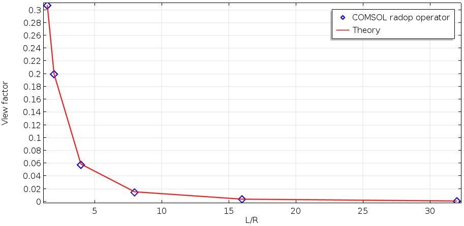
Comparison between the classical theory and the radopu operator calculation in COMSOL Multiphysics for the ambient view factor.

Now, let’s move on to the settings. To calculate surface-to-surface radiation, a Surface-to-Surface Radiation physics interface and a Diffuse Surface node for the internal surface of the sphere need to be added, and a Heat Transfer with Surface-to-Surface Radiation multiphysics coupling node needs to be added (see below). COMSOL Multiphysics will compute the view factor by performing surface integration for each mesh node except when the geometry is axisymmetric where a closed-form expression is used. For the sake of simplicity, we don’t include ambient radiation; i.e., T_{\rm amb}=0. A Temperature boundary condition is set to the outer boundary of the spherical shell with T_0 = 2500 deg K. The material emissivity is set to 0.5 in order to see the difference more easily.

Settings for the Diffuse Surface node.

The following plots show the computed ambient view factor, radiosity, and temperature for various opening radii. Following Gouffé’s paper, the geometry aspect ratio defined by L/R, where R is the opening’s radius and L is the cavity height, is used as a sweep parameter.

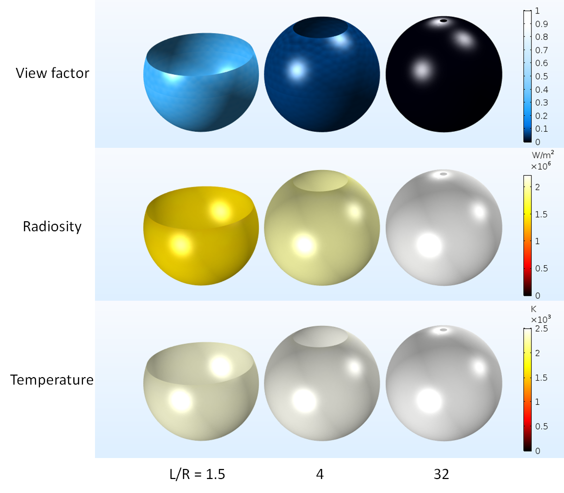
Computational results for the ambient view factor, radiosity, and temperature versus L/R.

These results qualitatively suggest that the smaller the size of the opening, the more the cavity emits thermal radiation and the higher the surface temperature.

To calculate the apparent emissivity for the computed radiosity result, we can now use the Stefan-Boltzmann law. The radiosity of the black body at temperature T_0 is \sigma T_0^4. Dividing the computed radiosity by this number, we get the apparent emissivity of the gray body spherical cavity, which is intop1(ht.J)/intop1(1)/(sigma_const*T0^4). Let’s now compare the results with the various theories we have discussed so far.

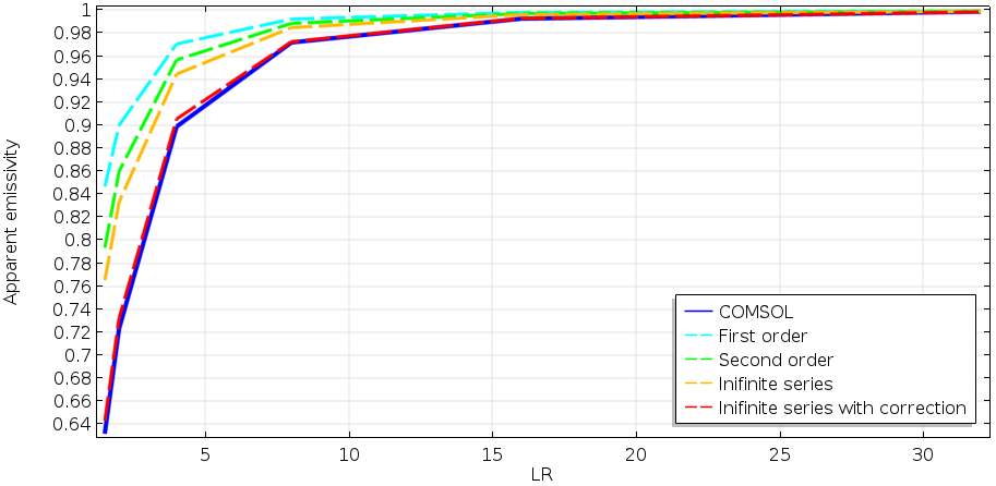
Comparison between COMSOL Multiphysics results and various theoretical approximations for the apparent emissivity for a spherical cavity.

The cyan line shows the first-order approximation, which underestimates the amount of reflection causing the higher emissivity, which is inaccurate. The second order obviously improves the accuracy, but it’s not enough. The plot for the infinite series approximation (orange line) gives a much better result, but it’s still not very close to the COMSOL Multiphysics results.

The reason for this discrepancy is mentioned in the last part of Gouffé’s paper. As some readers might have noticed in the previous figure, the surface temperature is different for each geometry, regardless of the same outer boundary temperature of 2500 deg K. This is called radiation cooling. We have yet to include this effect, which takes place for any real material with a finite thermal conductivity. The effect changes the temperature of the inner surface of the shell temperature, depending on the opening area. Therefore, the temperature needs to be compensated in order to calculate the emissivity at the same temperature for all opening areas.

The correction factor is, owing to the Stefan-Boltzmann law, the fourth power of the temperature ratio; i.e., (maxop1(T))^4/T0^4, where maxop1 is an operator defined on the cavity surface that finds the maximum value on the surface. Finally, with this correction, the red curve is the most accurate theoretical prediction, which agrees very well with the COMSOL Multiphysics results (blue line).

Designing an Efficient Incandescent Lamp with the COMSOL® Software

The light source in an incandescent lamp is created by a twisted tungsten filament. The material emissivity of tungsten is 0.462 at 2500 deg K for a 0.467-um wavelength (Ref. 2). In the past, researchers proposed that we can design more efficient incandescent lamps if we fabricate some microstructures on the surface of the tungsten filament. This is true. As we just learned, the apparent emissivity can be close to 1 if we have a cavity with a very tiny opening, which we can call a black body filament. In addition, research (Ref. 3–4, 8–9) also proposed that if the maximum cavity size is about a half of 0.78 um, then any infrared light with a wavelength larger than 0.78 um may be suppressed due to the waveguide’s cutoff effect. Then, the efficiency for the visible light may be significantly improved.

This effect may be more than the emissivity enhancement, because thermal radiation below tungsten’s melting temperature consists of mostly infrared light that is wasted to heat. It would be fantastic if we could really cut the infrared off.

Our “dream” incandescent lamp with an infrared suppressing black body filament. Background image in the public domain, via Wikimedia Commons.

Unfortunately, this “dream lamp” can’t be a reality for various reasons.

First, it isn’t possible for the surface to be made up of “all” holes. To make holes with a low view factor, meaning a smaller opening area than the hole size, the surface can’t be densely filled with the openings; i.e., the surface needs a flatter area between the openings, which radiate infrared. Alternatively, we can make deep holes to decrease the ambient view factor and then make each hole as close to the adjacent holes as possible. However, this makes it more difficult to fabricate deeper holes.

Also, the surface energy of the surface with holes seems to be higher than that of a flat surface. So, the surface with holes tends to melt down at a lower temperature than the bulk melting temperature.

Third, it is very difficult to make holes on a twisted wire filament because it’s a 3D structure. It is easier to make holes on a flat ribbon filament because it’s 2D, but flat filaments are not electrically convenient because they need more current to achieve the same temperature than the twisted wire filament (higher voltage and lower current is convenient for our current infrastructure).

Concluding Remarks

Although gray body radiation theory was developed a long time ago, the theory is still well organized. There are many sources for closed-form view factor formulas (Ref. 5; note that it’s also called “configuration factor”). This theory has been proven by experiments and is still applied to many real-world applications, but it can seem too difficult to understand. In this blog post, we learned the theory for the simplest example and saw a very successful benchmark result with COMSOL Multiphysics. The Heat Transfer with Surface-to-Surface Radiation interface is a reliable tool that makes complicated radiation computations easier.

We can come up with a more interesting incandescent lamp by making a special view factor. If we make tiny periodic grooves on a flat ribbon filament, we will get a “directional” incandescent lamp. Usually, a filament emits light to all directions, but this special filament illuminates only a certain direction (Ref. 6). We can explore many more ideas and many more applications of gray body radiation theory with simulation.

Next Step

Try the Gray Body model yourself by clicking the following button, which will take you to the Application Gallery. There, you can download the related MPH-file.

References

1. A. Gouffé, “Corrections d’ouverture des corps-noirs artificiels compte tenu des diffusions multiples internes (Corrections of emissivity for the artificial black-body considering multiple internal diffusions)” (in French), Revue d’Optique, t. 24, no. 1–3, 1945.
2. C.J. Smithells, Tungsten, Chapman & Hall, Ltd., 1926.
3. J.F. Waymouth, Proceedings of LS-5, 1989.
4. J.F. Waymouth, J. Illum. Engng. Inst. Jpn., 74, 12, pp. 800–805, 1990.
5. J.R. Howell, “A Catalog of Radiation Heat Transfer Configuration Factors“, University of Texas at Austin.
6. W.Z. Black, “Radiative heat transfer characteristics of specially prepared V-groove cavities”, PhD Thesis to Purdue University, 1968.
7. Precision Measurement and Calibration, Radiometry and Photometry (Vol. 7), U.S. Department of Commerce, National Bureau of Standards.
8. M. Sugimoto, T. Fujioka, T. Inoue, H. Fukushima, Y. Mizuyama, S. Ukegawa, T. Matsushima, and M. Toho, “The Infrared Suppression in the Incandescent Light from a Surface with Submicron Holes”, Journal of Light & Visual Environment, Vol. 18, No. 2 (1994).
9. T. Kondo, S. Hasegawa, T. Yanagishita, N. Kimura, T. Toyonaga, and H. Masuda, “Control of thermal radiation in metal hole array structures formed by anisotropic anodic etching of Al”, Optics Express Vol. 26 No. 21 (2018).