
The viscous catenary problem has generated a lot of theoretical and experimental interest in recent years. This is due to the industrial importance of the rich phenomena that occur within it. Using the flexibility of the COMSOL Multiphysics® software, we can gain fundamental insights into complex problems like the viscous catenary problem and determine the validity of the assumptions made in previous analyses.
The Historical Significance of the Catenary Curve
In the fields of mathematics and physics, the catenary curve has a historical significance. Not only does it highlight the relationship that exists between geometry and mechanics, but it also plays an important role in structural engineering.
Catenary, which comes from the Latin word for “chain”, describes the curve-like shape assumed by an idealized chain or cable that hangs beneath its own weight from supports at each end. Robert Hooke, an English scientist and architect, studied the properties of this geometric shape in the 1670s. During this time, he realized that the curve represents the optimal form of an arch with a constant cross section. While Hooke knew that the catenary shape was different than a parabola, it wasn’t until 1690 that other researchers determined its mathematical form.

Robert Hooke holding a chain that forms a catenary curve. Image by Rita Greer. Licensed under Free Art License 1.3, via Wikimedia Commons.
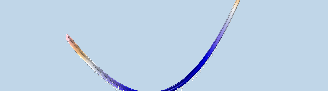
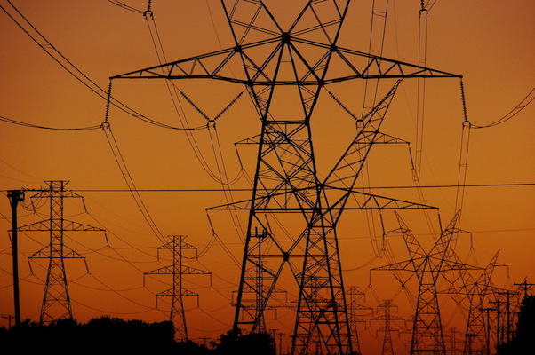
Today, catenary curves are found in a variety of structures, such as free-hanging electrical cables and suspension bridges. Meanwhile, many arches follow an inverted catenary curve, where the shape of the hanging chain acts as a guide for material placement. By pushing gravity’s vertical forces into compression forces throughout the arch’s curve, these designs are able to withstand their own weight.

Top: Free-hanging cables follow the catenary curve. Image by Loadmaster (David R. Tribble). Licensed under CC BY-SA 3.0, via Wikimedia Commons. Bottom: Many other structures use an inverted configuration of the curve, including the arches in the Sheffield Winter Garden. Image in the public domain, via Wikimedia Commons.
Exploring the Viscous Catenary Problem
Up to this point, we’ve discussed the catenary curve as it relates to a solid material. But what happens when the material is a fluid? This type of problem can be a bit more complicated to address.
The viscous catenary problem describes how a cylinder composed of a highly viscous fluid moves as it flows beneath gravity, supported at both ends. The rich phenomena that occur within this process have industrial importance in various applications, including glass manufacturing and filament spinning. For this reason, the study of the viscous catenary problem has garnered quite a bit of theoretical and experimental interest in the academic field.
In the past, researchers have provided 1D solutions for the viscous catenary problem (see the references in the model documentation). To gain further insight into the problem and address the validity of the assumptions made in previous research, we can run our own simulation tests in COMSOL Multiphysics. Let’s examine a tutorial from the Microfluidics Module that explores this problem.
Designing a Model to Investigate the Phenomena in the Viscous Catenary Problem
The viscous catenary model is comprised of a cylinder of Newtonian fluid that falls beneath its own weight. Its design is characterized by the following properties:
- Initial diameter: 0.6 mm
- Length: 21.5 mm
- Fluid density: 1000 kg/m3
- Viscosity: 100 Pa·s
The fluid inside of the structure has a surface tension of 22 mN/m.
With regards to the flow, the capillary number is high. This makes the contact angle between the fluid and the cylinder’s supporting surfaces unimportant. As such, we apply a nominal value of 90º. Further, adding a Navier Slip boundary condition to each surface enables slight movement of the cylinder’s supporting edges. Compared to the overall displacement of the cylinder, this displacement is rather small and can be omitted from the results as needed.
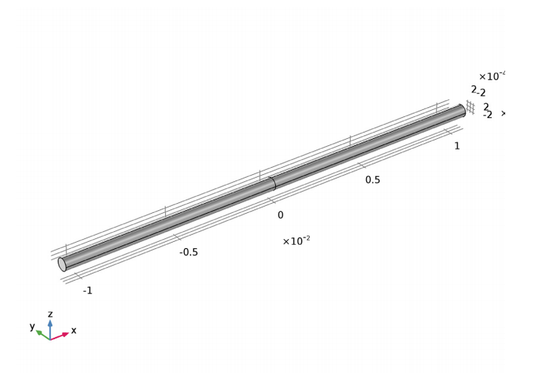
The model geometry.
As highlighted above, the cylinder is split into two halves so that points can be set up at the center of the structure. We then use these points to compute the height of the catenary’s lowest point.
Evaluating and Comparing Simulation Results
After two seconds of falling, the fluid velocity of the catenary is measured. The results indicate that the fluid velocity is primarily vertical. Looking at the pressure inside the curve, variations are most prevalent in the small area next to the anchors. This is the point at which the radius of the surface’s curvature is greatest.


The fluid velocity (left) and pressure (right) inside the catenary.
The next plot shows the position of the catenary’s centerline as a function of time at 0.02-s intervals. The parabolic profile is apparent for the central part of the catenary’s length. The 1D theory for intermediate time scales predicts such an effect.
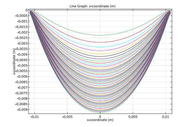
The position of the catenary’s centerline.
We can observe the vertical distance between the center of the catenary and its anchors as a function of time. The simulation results are then compared with experimental data (Ref. 2 in the model documentation). The agreement between the two falls within experimental error. Note that this doesn’t include the scaling factor used in previous research to obtain agreement with the presented theory. Performing another parametric sweep on the surface tension coefficient indicates that this scaling factor is related to surface tension — an element that is neglected in the previous theoretical treatments.
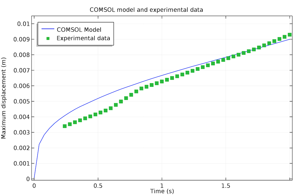
A comparison of the simulation and experimental results for the displacement of the catenary’s center as relative to its anchors.
This example is a good representation of using COMSOL Multiphysics to gain fundamental insights into complex problems. Through the flexibility of the software, we can solve problems without having to use assumptions, which in turn enables us to address the validity of assumptions from previous simplified studies.
Learn More About Simulating Microfluidics Problems with COMSOL Multiphysics®
- Browse all of the blog posts within the Microfluidics category
- Try other tutorials from the Microfluidics Module:


Comments (0)