Taking Care of Fast Oscillations with the Wave Optics Module

The new COMSOL Multiphysics Wave Optics Module provides engineers with a great set of features for designing their simulations. One of the new capabilities included in this module is the groundbreaking beam envelope method for electromagnetic full-wave propagation. We hope this feature will become instrumental to the optics community.

Beam Envelope Method

When attempting to simulate electromagnetic wave propagation in optical waveguide structures, such as optical fibers, engineers are faced with a seemingly unsolvable problem: the electromagnetic waves are oscillating rapidly in the direction of propagation. For standard computational methods (such as the finite element method) to handle such cases efficiently, they require a very fine mesh, much smaller than the wavelength. Enter the beam envelope method. This method provides a clever way of capitalizing on the fact that in optical components you often have a well-defined single direction of propagation. Instead of solving for the incredibly computationally-intensive electric field, you solve for the slowly varying electric field envelope.

Solving directly for the electric field requires the oscillations to be resolved with sample points that are dense enough to avoid aliasing. The Nyquist–Shannon sampling theorem tells us that you need at least three sample points per wavelength to resolve the wave. With numerical methods for electromagnetic wave propagation, you usually need even more than three sample points, or discretization points, per wavelength. This is due to technical reasons surrounding the numerical scheme used. The finite element method is one method offered by COMSOL to solve for electromagnetic field propagation. Using finite element terminology, it is recommended that you have a least five quadratic finite elements per wavelength. By instead solving for the slowly varying field envelope, we get by with a lot fewer sample points; that is, a much coarser mesh can be used.

Built into this method is a factorization trick — you separate out the fast-varying portion of the wave as illustrated in the picture above: 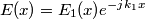. The user provides the wave-vector k₁ as an input to the method. To recover the “real” field you just multiply the solution E₁(x) with the fast-varying phase factor. The picture below illustrates the difference between the sample density for the electric field and the electric field envelope.

The simulations you can perform with this new method are quite impressive, especially considering that there are no particular approximations involved other than that of the applied finite element method using vector (also known as edge, or Nedelec) elements.

The picture above (top) shows the true aspect ratio representation of a self-focusing laser beam simulation and (bottom) a compressed view with the variation in refractive index as an isosurface.

Wave Optics Module

The beam envelope method is one of the main features of the new Wave Optics Module that was released May 3^rd with COMSOL Version 4.3b. The method, as implemented in the module, comes in two flavors: unidirectional and bidirectional. The bidirectional method actually solves for two waves: one incident and one reflected. In optical devices you may very well get reflections back the same direction the wave originated in and the bidirectional method is designed for that case. The beam envelope method complements the conventional electromagnetic full-wave propagation methods that are also featured in the Wave Optics Module. These user interfaces are very similar to those of the RF Module but are tailored for optics simulations, having the refractive index as the default option rather than the permittivity default of the RF Module.

The Wave Optics Module gives you several analysis options including 2D, 3D, frequency-domain, eigenfrequency, and time-domain simulations. We anticipate that it will be used for wave propagation through optical media including engineered metamaterials and gyromagnetic materials. It has built-in support for anisotropic permeability, permittivity, and refractive index tensors, with or without losses.

As you may know, COMSOL Multiphysics has been used for quite some time by the optics community. The Wave Optics Module expands on previous capabilities of COMSOL Multiphysics and the RF Module, and it is the first dedicated optics product we have released. Tune into our free Wave Optics Simulations webinar on June 13^th to learn more.

Further Reading

• Plasmonic Properties of Bimetal Nanoshell Cylinders and Spheres