Blog Posts Tagged Technical Content
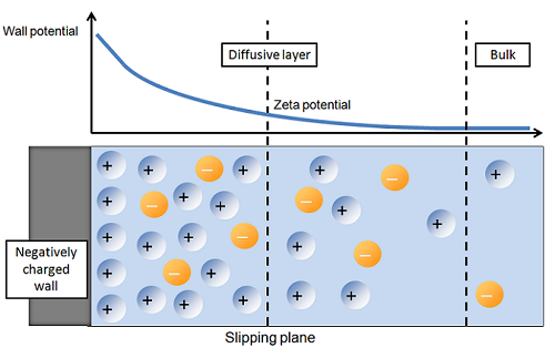
Modeling Electroosmotic Flow and the Electrical Double Layer
Microfluidic devices are so small that the micropumps and micromixers that control and mix the fluid inside the device cannot involve any moving components. Instead, they must take advantage of electroosmotic flow. Here, I will describe the concept of electroosmosis and the electrical double layer (EDL), and how to model these in COMSOL, walking you through two example models.
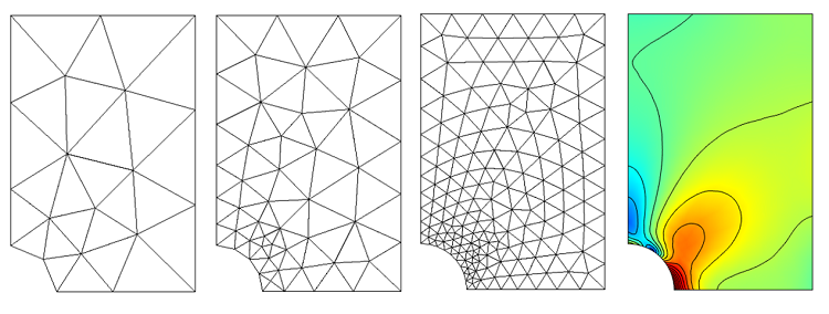
Meshing Considerations for Linear Static Problems
In this blog entry, we introduce meshing considerations for linear static finite element problems. This is the first in a series of postings on meshing techniques that is meant to provide guidance on how to approach the meshing of your finite element model with confidence.
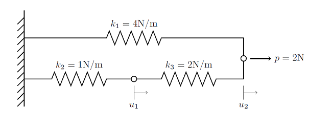
Solving Linear Static Finite Element Models
In this first blog entry of our new solver series, we describe the algorithm used to solve all linear static finite element problems. This information is presented in the context of a very simple 1D finite element problem, but is applicable for all cases, and is important for understanding more complex nonlinear and multiphysics solution techniques to be discussed in upcoming blog posts.
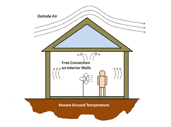
Using Global Equations: Modeling Room Air Temperature in a House
An interesting question came up the other day that I felt would make an excellent blog post since it allows us to discuss one of the very powerful, and often underutilized, features of COMSOL Multiphysics: the Global Equation. In this post, we will look at using global equations to introduce an additional degree of freedom to a model. This additional degree of freedom will represent something we do not want to model explicitly.
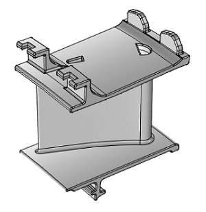
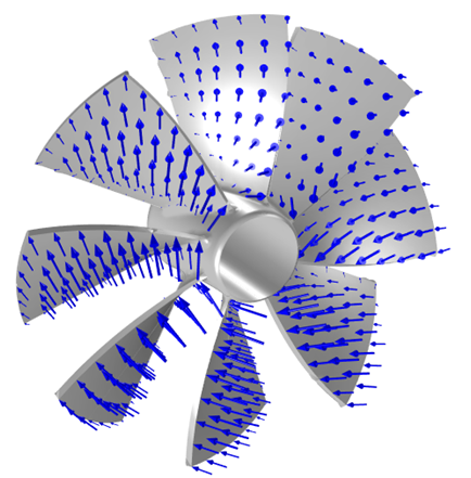
Simulating Thermal Stress in a Turbine Stator Blade
We can leverage simulation software to understand and optimize component design. Every simulation relies on a model that is a representation of the reality that the application finds itself in. Modeling enables us to represent this reality with enough detail to receive relevant information about the particular application or component. Let’s have a look at a thermal stress analysis of the turbine stator blade model from our Model Gallery and investigate the effects of heat transfer and thermal stress that […]

Modeling Magnetostriction Using COMSOL Multiphysics®
If you have ever stood next to a transformer, you have probably heard a humming sound coming from it and wondered if there were bees close by. When you hear that sound the next time, you can rest assured that it’s not bees but the magnetostriction of the transformer core that is making that humming sound.
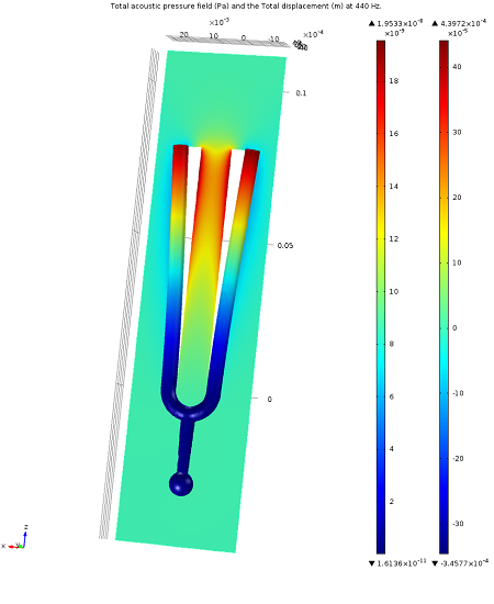
Tuning an Orchestra with the Help of Multiphysics Simulation
Multiphysics applications are all around us. Consider, for example, a setting where science may be the last thing on our minds: a music concert. You might be enjoying the slight sinusoidal variations in atmospheric pressure we call sound waves, or music, but those pressure variations must come from somewhere. In fact, they are due to a multiphysics effect where sinusoidal structural vibrations in an object disturb the surrounding air, causing pressure variations in the air that then propagate outward and […]
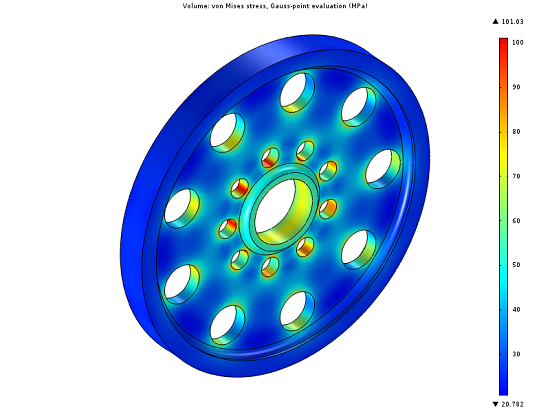
Using Gradient-Free Optimization
The COMSOL Optimization Module includes both gradient-based and gradient-free optimization techniques. Whereas the gradient-based optimization method can compute an exact analytic derivative of an objective function and any associated constraint functions, it does require these functions to be smooth and differentiable. In this blog post, we examine the use of the gradient-free optimizer, which can consider objective function and constraints that are not differentiable or smooth. The dimensions of a spinning wheel are optimized to reduce the mass while maintaining […]
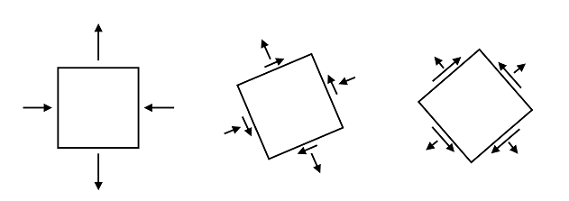
Fatigue Prediction Using Critical Plane Methods
Research on fatigue started in the 19th century, initiated following failing railroad axles that caused train accidents. In a rotating axle, stress varies from tension to compression and back to tension in one revolution. The load history is simple because it is uniaxial and proportional. Fatigue can then be evaluated with the S-N curve, also known as the Wöhler curve, which relates stress amplitude to a component’s life. In many applications we deal with multiaxiality and non-proportional loading. In this […]
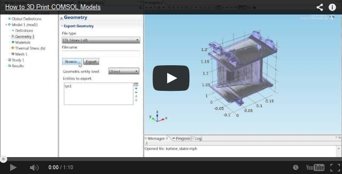
How to 3D Print COMSOL Models
Quite often we get asked the question “can I 3D print my COMSOL model?” Well, as of version 4.3b, the answer is “yes!” This is because it is now possible to export geometries and meshes as STL files, which is one of the standard file formats for 3D printing. This allows for rapid prototyping of designs; there is no need to outsource parts to machine shops. It is quite remarkable that you could conceive, simulate, optimize, and prototype a design […]
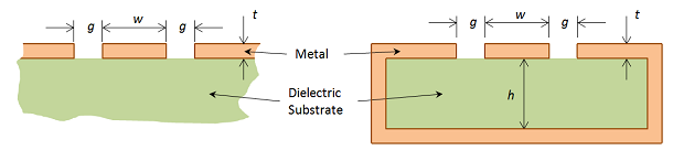
Modeling of Coplanar Waveguides
The Coplanar Waveguide (CPW) is commonly used in microwave circuits. COMSOL Multiphysics, with the RF Module, makes it easy to compute the impedance, fields, losses, and other operating parameters needed when designing a CPW.
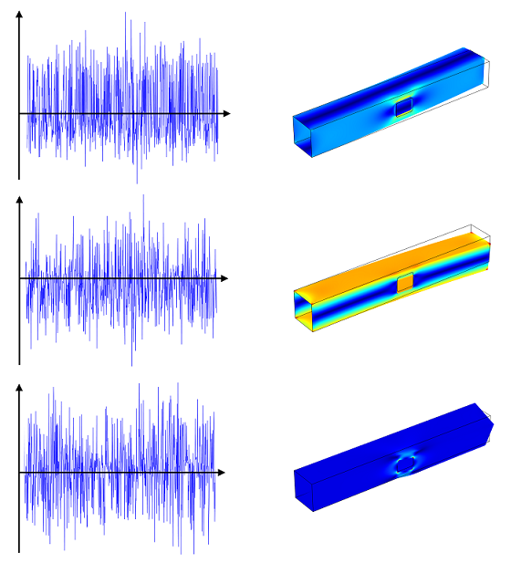
Random Load Fatigue
In many applications, loads applied to structures are random in nature. The sampling results of the structural response will differ depending on the data collection time. Although the stress experienced is not always high, the repeated loading and unloading can lead to fatigue. The engineering challenges in these types of applications are defining the stress response to the random load history in the critical points, and predicting fatigue damage. This is simulated with the Cumulative Damage feature in the Fatigue […]
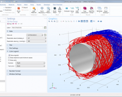
Using Curvilinear Coordinates
Curvilinear coordinates are a coordinate system where the coordinate lines may be curved. The new user interface for automatic computation of curvilinear coordinates is a very practical addition to version 4.3b for those working with anisotropic materials in free-form CAD designs. If you have a generic bent shape and try to apply the usual coordinate systems like Cartesian, cylindrical, or spherical, you are out of luck. Curvilinear coordinates are needed to smoothly follow the design, which typically has no mathematical […]
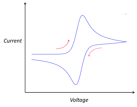
Modeling Electroanalysis: Cyclic Voltammetry
If you’re not an electrochemist, chances are you’ve never come across cyclic voltammetry. But look at any electrochemical journal, conference proceedings, or company website for manufacturers of electrochemical sensors. Somewhere near the front, you’ll see a distinctive “double-peaked” graph.
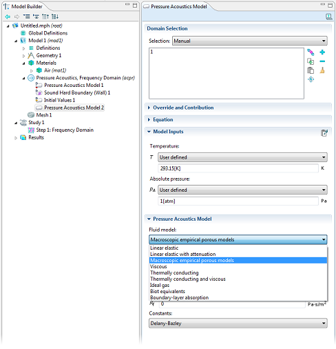
Modeling Acoustic Damping Processes
Mufflers are often located in exhaust systems or on heat, ventilation, and air conditioning (HVAC) systems, where their key functionality is to dampen the noise that is emitted from the system. A correct description of the acoustic damping (absorption and attenuation) processes in the muffler is important when designing and modeling these systems.
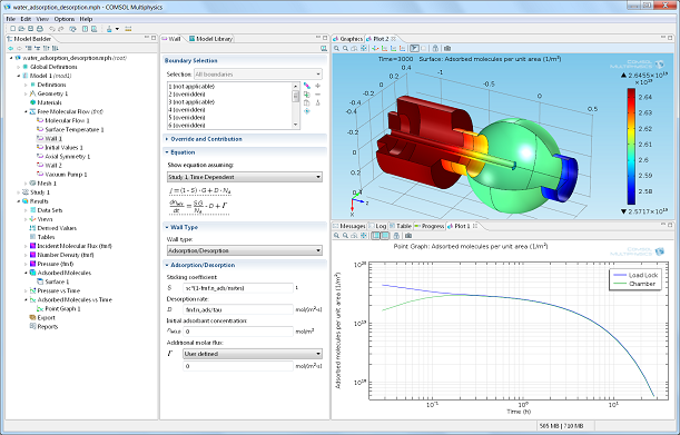
Molecular Flow Module: Simulate Rarefied Gas Flows in Vacuum Systems
Vacuum technology has many important applications, from semiconductor device and MEMS fabrication, to vacuum coatings for corrosion protection, optical films, and metallization. The new Molecular Flow Module provides vacuum engineers with previously unavailable tools for modeling gas flows within vacuum systems.
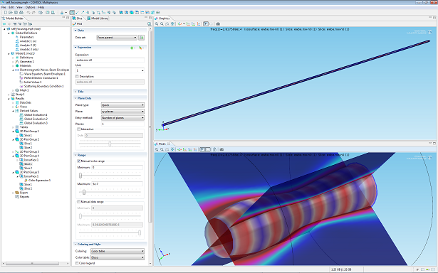
Taking Care of Fast Oscillations with the Wave Optics Module
The new COMSOL Multiphysics Wave Optics Module provides engineers with a great set of features for designing their simulations. One of the new capabilities included in this module is the groundbreaking beam envelopes method for electromagnetic full-wave propagation. We hope this feature will become instrumental to the optics community.
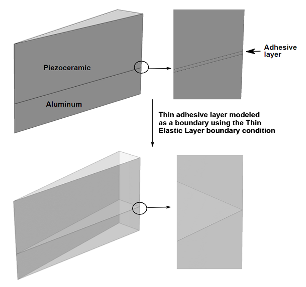
Structural Analysis with Thin Elastic Layers
Some structural applications involve thin or high aspect ratio structures sandwiched between other relatively low aspect ratio structures. For example, if a piezoelectric transducer is glued on the surface of a mechanical system, the thickness of the adhesive layer is very small in comparison to the two structures it glues together. Numerical modeling of such a thin layer in two or three dimensions requires resolving it with an appropriate finite element mesh. This can result in a large concentration of […]
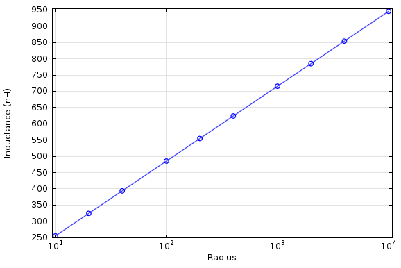
Computing the Inductance of a Straight Wire
A question that comes up occasionally is whether or not you can compute the inductance of a single straight wire. This seemingly simple question actually does not really have an answer, and gives us the opportunity to talk about a very interesting point when solving Maxwell’s equations. Anybody working in the field of computational electromagnetics should have an understanding of this key concept, as it will help you properly set up and interpret models involving magnetic fields.
Using Point Cloud Data in Your COMSOL Model
There is sometimes a need to include data from other simulation packages into a COMSOL Multiphysics model. There are a variety of ways in which this can be done, but one of the easiest approaches is to read in the point cloud data via a spreadsheet format text file. In this blog post, we walk through the steps of reading in such data, and using it in a COMSOL model.

Probing Your Simulation Results
For a transient simulation, imagine if you could simply insert a virtual sensor in a model at a certain location and then monitor the evolution of a field value over time while solving. In COMSOL Multiphysics® you can do just that by using Probes. You define a probe in the Model Builder tree right under the Model Definitions node. Measuring the value at a point is not the only thing you can do with probes, but in this blog post we […]
Acoustofluidic Multiphysics Problem: Microparticle Acoustophoresis
The use of acoustic waves to manipulate suspensions of particles, such as cells, has inspired the work of many researchers, paving the way for the field of ultrasound acoustofluidics. The manipulation is achieved in many ways, including using bulk acoustic waves (BAW) and surface acoustic waves (SAW), as well as acoustic radiation forces and acoustic streaming-induced drag. The latter two combine to produce the acoustophoretic motion of the suspended particles; i.e., movement by means of sound, and the methods provide […]
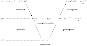
On Solvers: The V-Cycle Multigrid
As discussed previously on the blog, iterative methods efficiently eliminate oscillatory error components while leaving the smooth ones almost untouched (smoothing property). Multigrid methods, in particular, use the smoothing property, nested iteration, and residual correction to optimize convergence. Before putting all of the pieces of this proverbial puzzle together, we need to introduce residual correction and dive a bit deeper into nested iteration. Let’s begin with the latter of these elements.
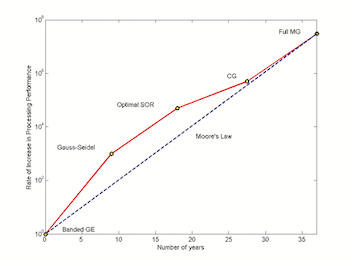
On Solvers: Multigrid Methods
Solution methods are a valuable tool for ensuring the efficiency of a design as well as reducing the overall number of prototypes that are needed. In today’s blog post, we introduce you to a particular type of method known as multigrid methods and explore the ideas behind their use in COMSOL Multiphysics.