

In a recent webinar, I highlighted how SmartUQ®, a predictive analytics and uncertainty quantification (UQ) software tool set, enhances product development and design exploration activities within the COMSOL Multiphysics® software. This blog post will further discuss how to incorporate COMSOL Multiphysics into your analytics workflow.
Predictive Analytics of SmartUQ® and UQ Workflow
The predictive analytics and UQ workflow shown below ties together SmartUQ® and COMSOL Multiphysics®. Our goal is to arrive at Step 5, where we can conduct analytics and uncertainty quantification. However, the analyses shown in Step 5, such as sensitivity analysis, uncertainty propagation, and optimization, rely upon a large quantity of samples to be effective. This is true of many advanced analytics techniques.
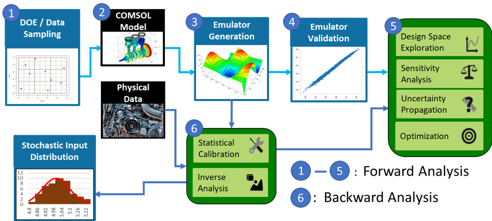
The challenge is the high computational cost of running the simulation at so many input configurations. The solution is to build an accurate predictive model, called an emulator in SmartUQ®, that can rapidly predict the output of our simulation for any set of inputs.
An emulator is a statistical model that utilizes machine learning algorithms to learn the input/output relationships of an underlying dataset, called the training data. In our case, the training data would be a set of runs from the COMSOL model. Once the emulator has been trained, we can use it to rapidly predict for whatever analytics technique we wish to employ. To select the best set of training data for an accurate emulator, a design of experiments (DOE) in Step 1 may be constructed in SmartUQ® by selecting from one of several modern, space-filling design options.
To recap, in Step 1, we pick the best set of COMSOL simulation configurations to run. In Step 2, the simulations are run in COMSOL Multiphysics. The simulation data are used in Step 3 as training data to build the emulator. In Step 4, we validate the emulator’s accuracy to check that its predictions agree well with the COMSOL simulation it emulates. Once validated, we move to Step 5 to conduct analytics using the emulator’s predictions.
In the backward analysis portion of the process flow, we have statistical calibration, a very useful technique that incorporates physical or experimental data.
In statistical calibration, we make our emulator more accurate by utilizing physical or experimental data to tune parameters in the simulation model to better agree with the physical data. In statistical calibration, some amount of model form error is assumed. The statistical calibration in SmartUQ® not only tunes the calibration parameters but also models the discrepancy between the physical data and simulation model. We can use the discrepancy model to check for model form error. This technique allows us to calibrate a highly inaccurate simulation model and use the discrepancy model to reduce the model form error.
Example of COMSOL Multiphysics® in the UQ/Predictive Analytics Workflow
For the remainder of this post, let’s look at an example of how the predictive analytics and UQ workflow in SmartUQ® works with simulation models in COMSOL Multiphysics®.
Predictive Modeling of a Microwave Ablation of Hepatic (Liver) Cancer Simulation Model
Simulation
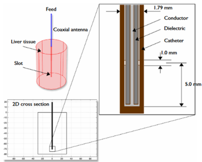
Microwave ablation is a form of thermal ablation for treating cancer by heating the tumor to cause necrosis (cell death). For a specific wattage used and treatment time, patient differences can affect the volume of necrotic tissue resulting from the procedure. The simulation model is a 2D cross section of tissue volume in COMSOL Multiphysics. The output is spatial data for percentage necrotic (dead) tissue after 7.5 minutes at 50 watts.
SmartUQ® Workflow
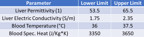
A 400-point DOE created in SmartUQ varies four patient-specific parameters within the bounds shown in the table below. With the results from COMSOL Multiphysics, we build a spatial temporal emulator in SmartUQ® to maintain the 2D feature of the dataset.
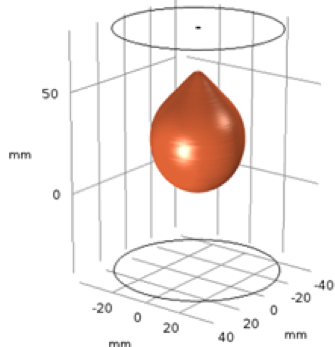
The plots in the figure below show the percentage of necrotic tissue for a given spatial point. There is strong agreement shown between the SmartUQ® prediction and the result directly simulated in COMSOL Multiphysics®. The SmartUQ® prediction takes approximately 30 seconds. By building the emulator for all points at once, the spatial emulation in SmartUQ® produces a smooth continuous surface allowing for analyses that wouldn’t otherwise be possible, such as the calculation of derivatives.
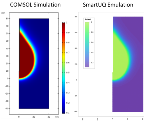
Comparison of a prediction made using the SmartUQ® spatial emulator with the result directly simulated in COMSOL Multiphysics®.
Next Steps
For a more in-depth look at the SmartUQ® workflow with COMSOL Multiphysics®, check out the white paper “SmartUQ Engineering Analytics Light-Weighting Application with COMSOL FEA Bracket Example” or our mini demo webinar with a COMSOL Multiphysics® simulation model.
About the Author
Gavin Jones, SmartUQ sr. application engineer, is responsible for performing simulation and statistical work for clients in aerospace, defense, automotive, gas turbine, medical device, and other industries. He is also a key contributor in SmartUQ’s digital twin/digital thread initiative. Mr. Jones received a BS in engineering mechanics and astronautics and BS in mathematics from the University of Wisconsin-Madison.
SmartUQ is a registered trademark of SmartUQ LLC.

Comments (0)