
Speaker drivers are electroacoustic transducers that make use of electromagnetic forces for generating vibration and radiating sound. Various types of drivers are available in the market, working under different principles. Here, we show the multiphysics coupling features that are built into the COMSOL Multiphysics® software for modeling speaker drivers.
Types of Speaker Drivers
Among all, the following four types of drivers form good representatives for the discussion of the physical mechanisms that are utilized in the design of the most well-known speaker drivers:
- Traditional dynamic transducers that use Lorentz force exerted on current-carrying voice coils to move the coils and the attached diaphragms. They are also known as moving-coil transducers, composing the most popular type seen nowadays.
- Balanced armature receivers that are primarily used in hearing aids and in-ear devices and the movement is induced by the Maxwell stress existing between magnetized bodies. They belong to a group called moving-iron speakers, which is the earliest type of electric loudspeakers to have been invented.
- Piezoelectric drivers that use piezoelectric materials, such as certain types of crystals that deform under the internal generation of a mechanical stress resulting from an applied electrical field. They are frequently used to generate sound in electronic devices and are also used as tweeters in some less expensive speaker systems.
- Electrostatic drivers that take advantage of electrostatic forces applied on large, thin, conductive diaphragm panels suspended between two perforated metal sheets. They have been popular with audiophiles due to the quality of low distortion and high clarity, and are usually more costly than the other types.
Although the driving forces behind all these speaker types belong to the category of electromagnetic forces, each has its own unique physical nature. Dynamic transducers and balanced armature receivers work in a magnetic field, and therefore modeling them in the COMSOL Multiphysics® software requires coupling the Solid Mechanics interface with the Magnetic Fields interface. On the other hand, piezoelectric drivers and electrostatic drivers work in an electric field, hence why it’s necessary to couple the Solid Mechanics interface with the Electrostatics interface.
COMSOL Multiphysics has the built-in multiphysics coupling features for modeling all four of these speaker drivers. Let’s take a closer look into each of them.
Lorentz Coupling
When a conductor sits in a magnetic field and is supplied with an electric current, an electromagnetic force, specified as Lorentz force, is exerted on it and causes it to move. On the other hand, the motion of the conductor through the magnetic field induces a voltage in it, a phenomenon known as the back EMF, which in turn affects the magnetic field. This is the working principle behind the conventional dynamic speaker drivers that use moving coils.
These moving-coil transducers contain permanent magnets for generating the magnetic field and coils placed in the magnetic field. When an AC voltage is applied to the coils, they move back and forth due to the varying Lorentz force, causing the connecting diaphragms to vibrate and radiate sound.
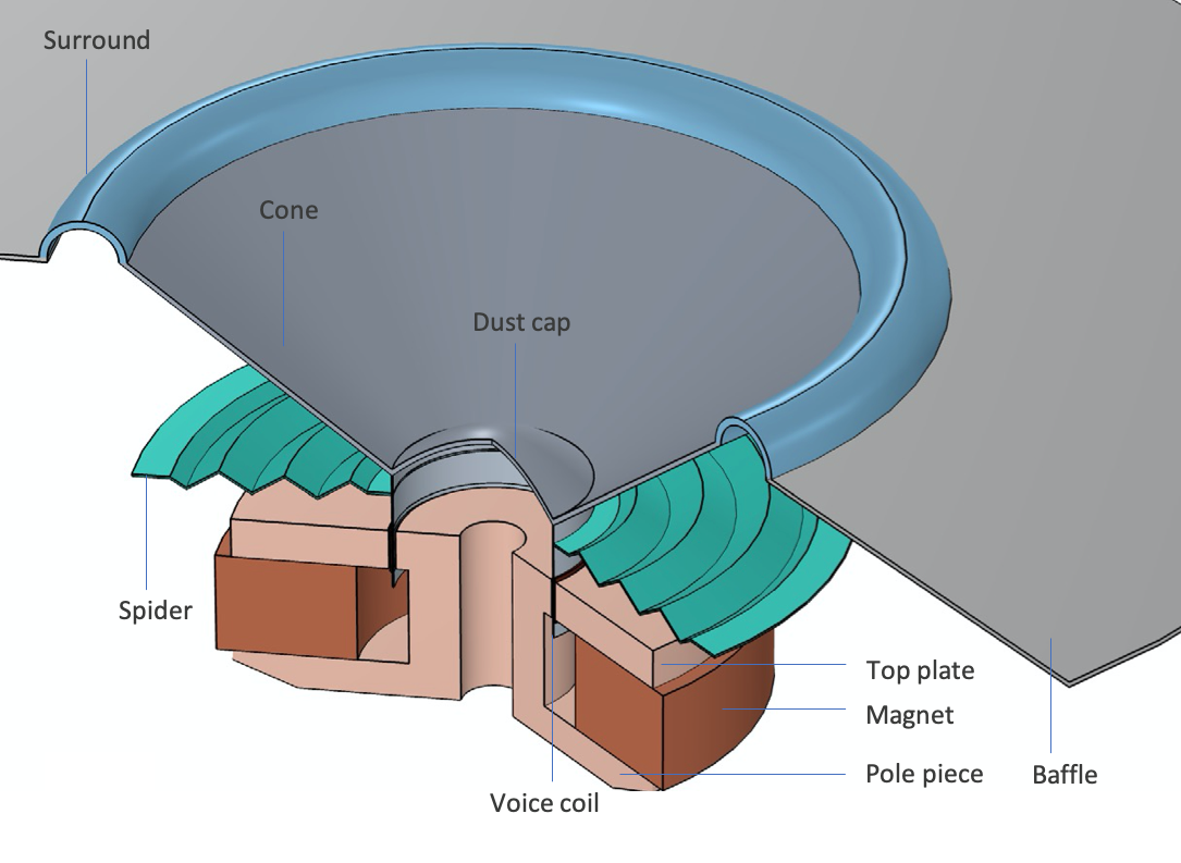
A moving coil transducer uses Lorentz force to induce vibration.
The Lorentz Coupling feature calculates the Lorentz force and back EMF to capture this two-way effect. It’s a multiphysics coupling feature between the Magnetic Fields interface and Solid Mechanics interface that passes the Lorentz force from the Magnetic Fields interface to the Solid Mechanics interface and passes the induced electric field from the Solid Mechanics interface to the Magnetic Fields interface. The Lorentz force and the induced electric field are calculated using these equations:
where \sigma is the electric conductivity, \textbf E is the applied electric field, \textbf v is the velocity of the moving coil, \textbf B is the magnetic flux density, and \textbf v\times \textbf B is the induced electric field. The total electric current density, \textbf J, includes contributions from both the applied electric field and the induced electric field and is used to calculate the Lorentz force, \textbf F.
When modeling loudspeaker drivers, the coupling is typically added in the voice coil domain, as shown in the Loudspeaker Driver — Frequency-Domain Analysis and Loudspeaker Driver — Transient Analysis tutorial examples.

The Lorentz Coupling feature is used to model a dynamic moving-coil transducer in the Loudspeaker Driver — Frequency-Domain Analysis tutorial example.
Magnetomechanical Forces
Balanced armature receivers are also made of magnets, coils, and diaphragms. However, they are operated under a completely different mechanism. In these devices, coils are fixed and do not move at all.
A single balanced armature receiver contains a small armature (arm) that is placed inside a voice coil and balanced between two magnets. When an AC current passes through the coil, it magnetizes the arm and puts it under the so-called Maxwell stress, the electromagnetic force existing between magnetized bodies. This force causes the armature to vibrate and move from one magnet to the other. As the arm is attached to the diaphragm, its vibrations are passed onto the diaphragm, which leads to the creation of sound waves.
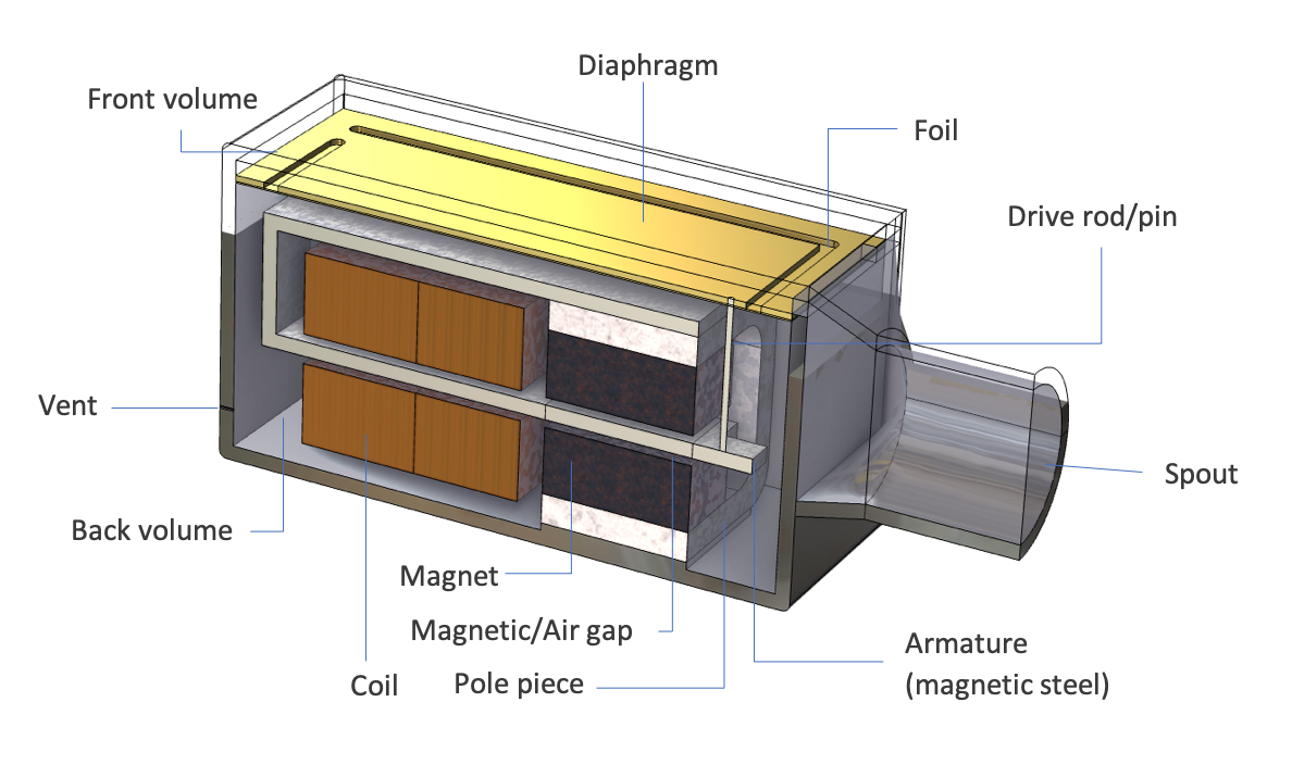
A balanced armature receiver that uses the Maxwell stress between magnetized bodies to induce vibration.
This is captured by the Magnetomechanical Forces coupling feature, another multiphysics coupling between the Magnetic Fields interface and Solid Mechanics interface. It’s used to calculate the Maxwell stress exerted on the magnetized deformable solids as well as the effect of structure deformations on material magnetization. The stress includes two components that contribute to deforming the solids: the stress that is present inside the magnetized bodies, and the stress that comes from the interactions with the surrounding magnetic field. The former is modeled as a body load, and the latter is applied as a boundary load on the solids’ exterior boundaries.
For finite deformations, the expressions for the electromagnetic stress and material magnetization in the solids can be derived using the following thermodynamic potential, called magnetic enthalpy:
where \mu_0 and \mu_r are the free space and relative magnetic permeability, respectively. The components of the magnetic flux vector, \textbf B, must be taken on the material frame, and the right Cauchy–Green deformation tensor is
\textup C=\textup F^{\textup T} \textup F, J=\textup{det}(\textup F)
with \textup F=\nabla \textbf u + \textup I, where \textbf u is the displacement field and \textup I is the identity tensor. The mechanical energy function W_s(\textup C) depends on the solid model used.
The total second Piola–Kirchhoff stress tensor is given by
and the magnetic flux density vector can be calculated as
The magnetic stress tensor is then calculated as
which is the so-called Minkowski magnetic stress tensor. This is applied as a body load to the solids.
The corresponding electromagnetic body force can be written as
This sometimes is referred to as the Korteweg–Helmholtz magnetic force, where \textbf J is the electric current and \chi=\mu_r-1 is the magnetic susceptibility, which can be a function of the mechanical strain in the material. This shows that the body force comprises both the Lorentz force and the force contribution from the magnetic polarization. The induction current effect is inherently included and is the sole contribution to the Lorentz force when there is no external current applied.
The boundary stress that is induced by the surrounding magnetic field, \sigma_{\textup E \textup M}^\textup{(out)}, is applied at the surfaces and is calculated as
where \textbf H and p are the magnetic field and the ambient pressure on the outer side of the solid boundaries.
COMSOL Multiphysics does not explicitly include the ambient pressure definition on the coupling features. However, it’s possible to add an additional surface force to the corresponding Solid Mechanics interface if the pressure is known or computed by another physics interface, for example, an acoustic model.
The use of the Magnetomechanical Forces Coupling feature is exemplified in the Balanced Armature Transducer tutorial model, as shown in the image below.

The Magnetomechanical Forces coupling feature is used in a full vibroelectroacoustic simulation of a balanced armature transducer.
Piezoelectric Effect
Piezoelectric drivers work because of the piezoelectric effect, a unique physical phenomenon present in certain crystalline materials, specified as piezoelectric materials. The direct piezoelectric effect consists of an electric polarization in a fixed direction when the piezoelectric crystal is deformed. The polarization is proportional to the deformation and causes an electric potential difference over the crystal. The inverse piezoelectric effect, on the other hand, constitutes the opposite of the direct effect. It describes the generation of deformation in the crystal when an electric field is applied, which is the mechanism behind piezoelectric drivers.
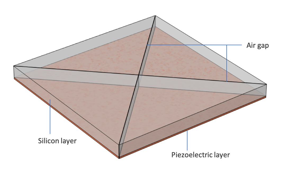
A piezoelectric MEMS speaker composed of four triangular membranes, which uses piezoelectric effect to induce vibration. A larger scale is applied in the thickness direction for visualization.
The direct and inverse piezoelectric effects are captured by the Piezoelectric Effect coupling feature, a multiphysics coupling between the Electrostatics interface and the Solid Mechanics interface. Each physics includes a dedicated piezoelectric material model, named Piezoelectric Material in the Solid Mechanics interface and Charge Conservation, Piezoelectric in the Electrostatics interface, to account for the specific constitutive relations in the piezoelectric domains. The two piezoelectric material models in the two physics are then coupled through the Piezoelectric Effect multiphysics feature. It’s possible to express the relation between the stress, strain, electric field, and electric displacement field in either a stress-charge form or a strain-charge form.
Stress charge:
Strain charge:
where \epsilon is the strain, \sigma is the stress, \textbf E is the electric field, and \textbf D is the electric displacement field. The material parameters c_E and s_E correspond to the material elasticity and compliance, e and d are the coupling properties, and \epsilon_0 and \epsilon_r are the free space and relative permittivity.
The Piezoelectric MEMS Speaker tutorial example demonstrates how to model a piezoelectric driver using the Piezoelectric Effect coupling feature.

The Piezoelectric Effect coupling feature is used in the Piezoelectric MEMS Speaker tutorial.
When it is necessary to run a transient analysis of sound radiation from a piezoelectric driver, there is an option to use the discontinuous Galerkin (dG or dG-FEM) method for modeling both vibrations of the piezoelectric device and wave propagation in fluids. In such a case, the Piezoelectric Waves, Time Explicit multiphysics interface is used to model the driver, which combines the Elastic Waves, Time Explicit interface and the Electrostatics interface together with the Piezoelectric Effect, Time Explicit multiphysics coupling. The dG formulation allows the fully coupled problem to be solved with an explicit time-stepping approach and thus provides an efficient alternative to model sound generation and propagation over large distances relative to the wavelength. This is explained in the Modeling Piezoelectricity Using the Discontinuous Galerkin Method blog post and demonstrated in the Ultrasonic Flowmeter with Piezoelectric Transducers tutorial example.
Electromechanical Forces
While electrostatic drivers also operate in an electric field, they use the Maxwell stress between charged bodies as the source for vibration. The diaphragm in these drivers is a thin, flat, conductive material, usually supplied with a constant charge on its surface. It’s sandwiched between two electrically conductive sheets called grids or stators. When an audio signal is applied to the grids out-of-phase, an electrostatic force is developed between the charged diaphragm and the grids on both sides. While one grid causes the diaphragm to push, the other causes it to pull, thus moving air and creating sound.
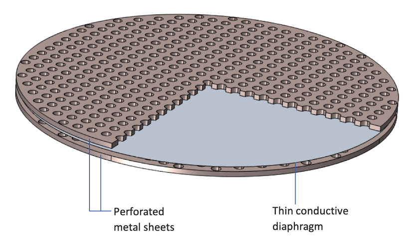
An electrostatic speaker driver, composed of thin plastic diaphragm residing between two perforated metal sheets, uses Maxwell stress existing between charged bodies to induce vibration.
This type of transducers can be modeled using the Electromechanical Forces coupling feature, another multiphysics coupling between the Electrostatics interface and the Solid Mechanics interface. It calculates the dielectric forces between the charged bodies, as well as the effect of the structure deformations on material polarization.
The theory is very similar to that of the Magnetomechanical Forces coupling, but the forces are now generated in an electric field rather than a magnetic field. There are also two contributing components: the stress that is generated inside the polarized dielectric bodies and modeled as a body load, and the stress that is induced by the surrounding electric field and applied as a boundary load on the surfaces.
For finite deformations, the expressions for the dielectric stress and material polarization can be derived using the following thermodynamic potential, called electric enthalpy:
where \epsilon_0 and \epsilon_r are the free space and relative permittivity. The components of the Electric Field, \textbf E, must be taken on the material frame, and the right Cauchy–Green deformation tensor is
\textup C=\textup F^{\textup T} \textup F, J=\textup{det}(\textup F)
with \textup F=\nabla \textbf u + \textup I, where \textbf u is the displacement field and \textup I is the identity tensor. The mechanical energy function W_s(\textup C) depends on the solid model used.
The total second Piola–Kirchhoff stress tensor is given by
and the electric displacement can be calculated as
The dielectric stress tensor is then calculated as
which is the so-called Minkowski electric stress tensor. This is applied to the body of the solids.
The corresponding electromagnetic body force can be written as
This sometimes is referred to as the Korteweg–Helmholtz electric force, where \rho_e is the electric charges and \chi=\epsilon_r-1 is the electric susceptibility which can be a function of the mechanical strain in the material.
The stress that is induced by the surrounding electric field is applied at the surfaces and is calculated as
where \textbf E and p are the electric field and the ambient pressure on the outer side of the solid boundaries.
COMSOL Multiphysics does not explicitly include the ambient pressure definition on the coupling features. However, it’s possible to add an additional surface force to the corresponding Solid Mechanics interface if the pressure is known or computed by another physics interface, for example, an acoustic model.
The Electrostatic Speaker Driver tutorial example demonstrates the use of the Electromechanical Forces coupling feature for simulating vibrations that are induced electrostatically.

The Electromechanical Forces coupling feature is used in the Electrostatic Speaker Driver tutorial to model the vibration of an electrostatically actuated diaphragm.
Adding an Acoustics Interface to Model Sound Radiation
Evaluating the performance of speaker drivers usually requires analyses of sound radiation to the surrounding fluids. You can then add an Acoustics interface and couple it to the solid vibrations model using the following coupling features:
- Acoustic-Structure Boundary: This feature is used to couple a pressure acoustics model to any structural component. This includes both the FEM-based acoustics interfaces and the BEM-based acoustics interface. The previously mentioned tutorials, the Loudspeaker Driver — Frequency-Domain Analysis, the Loudspeaker Driver — Transient Analysis, and the Balanced Armature Transducer, are examples of using FEM-based pressure acoustics interfaces. You can see an example of coupling BEM-based pressure acoustics interface with structure vibrations in the Loudspeaker Driver in a Vented Enclosure tutorial model.
- Acoustic-Structure Boundary, Time Explicit: This feature is dedicated for transient acoustic-structure interaction problems solved using the dG-FEM method with a time explicit solver. It is compatible with the Piezoelectric Effect, Time Explicit coupling feature for time dependent analyses of sound radiation from piezoelectric speaker drivers. See the Ultrasonic Flowmeter with Piezoelectric Transducers tutorial for a demonstration.
- Thermoviscous Acoustic-Structure Boundary: This feature is used to couple a Thermoviscous Acoustics interface with any structural component. A thermoviscous acoustics model is required to accurately simulate acoustics in narrow fluid channels when viscous losses and thermal conduction become important because a boundary layer exists. This is exemplified in the Piezoelectric MEMS Speaker and the Electrostatic Speaker Driver tutorial models.
There is also a pair version for each of the three coupling features: the Pair Acoustic-Structure Boundary coupling; the Pair Acoustic-Structure Boundary, Time Explicit coupling; and the Pair Thermoviscous Acoustic-Structure Boundary coupling. They are used to couple an acoustics interface to the Solid Mechanics interface in an assembly geometry where identity pairs have been created. This allows the use of nonconforming mesh at the acoustic-structure boundary. As the wave speeds differ in solids and fluids, the computational mesh can take advantage of this when resolving the waves. In this way you can save degrees of freedom when solving. The Pair Acoustic-Structure Boundary, Time Explicit coupling option is especially useful for dG-based models because of the need to avoid small internal solver time steps due to unnecessarily small mesh elements in a specific material domain, as explained in the Discontinuous Galerkin Method blog post.
Adding a Moving Mesh Feature for Large Deformations
In the case where the deformations of the structure are large and can significantly affect the electromagnetic field, either being electric or magnetic, a Moving Mesh functionality can be used to account for the effect of topology change due to structure deformations on the electromagnetic field distribution. This is demonstrated in the Electrostatic Speaker Driver tutorial example.
A moving mesh can also be used to capture the nonlinear effect due to the topology change in the acoustic field, generated by a speaker diaphragm with large deformations. The Loudspeaker Driver — Transient Analysis model uses the Moving Mesh feature and Automatic Remeshing to capture the topology changes and the movement of the voice coil.
Next Step
This blog post has discussed four available coupling features for modeling most commonly seen speaker drivers in the market. Explore the models mentioned here by downloading the documentation and MPH files from the Application Gallery:
- Loudspeaker Driver — Frequency-Domain Analysis
- Loudspeaker Driver — Transient Analysis
- Balanced Armature Transducer
- Piezoelectric MEMS Speaker
- Electrostatic Speaker Driver
Contact us if you want to learn which modules are required to have access to these coupling features.

Comments (2)
Acculution ApS
June 28, 2022Great post, Jinlan! Very important to understand these different transductance principles. Currently working on projects where all four principles are used.
Phanindra Reddy Ravi
October 20, 2022Nice blog, Thanks a lot.