
As of version 5.5 of the COMSOL Multiphysics® software, default plots have been added to all structural mechanics interfaces to show applied loads. In this blog post, we will discuss how you can work with these load plots to get the best possible visualization of the loads acting on your model in various situations.
Editor’s note, 12/12/22: In COMSOL Multiphysics version 6.1, predefined plots were introduced. In this version, the load plots are now predefined plots, which can be added on demand, unlike the always generated default plots.
How the Load Plots Are Structured
The load plots use the standard result visualization tools; mainly, vector plots.
For each study and physics interface, one set of load plots is generated. Since there can be many plot groups containing loads, they are always placed inside a group node in order to avoid overpopulating the Results branch in the model tree. The group node itself is labeled Applied Loads (interface_tag).
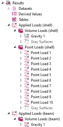
Example of load plots in a model containing two physics interfaces and a single study.
The subdivision into plot groups is dictated by the space dimension of the entity to which the load is applied. Since, for example, boundary loads and point loads have different physical units, it is not meaningful to plot them together with a common scaling of arrow sizes. Thus, the plot groups bear names like Volume Loads or Edge Loads. There is one notable exception to the rule about dimension: Volumetric loads, like gravity or rotating frames, are always considered as volume loads, even if applied to an edge in a Beam interface, for example.
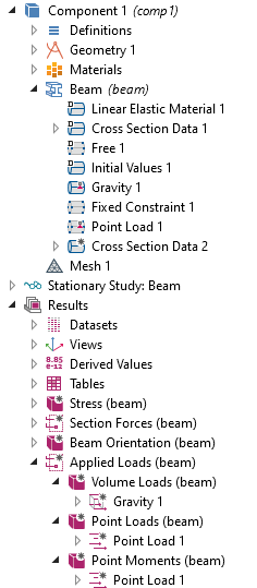
Within the plot group, each load feature in the physics interface will, in general, generate a plot node with the same label as the load node itself. If you add mnemonic labels for the loads, you will easily find the corresponding load under the plot groups.
There are some cases in which more than one plot node is generated from a single load feature. For example, moments and forces are separated into different plot groups, since they have different physical dimensions. Also, rotating frame loads are separated into centrifugal forces, Coriolis forces, and Euler forces.
In load features where you can enter both forces and moments, a special rule is applied: A plot node will always be created for the force, irrespective of its values. The corresponding node for the moment is, however, only generated when at least one of the moment components is not identical to zero.
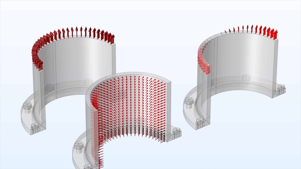
Load plots generated from a Beam interface. Note that the loads entered in the Point Load 1 node have been split into two plot groups; one for force and one for moment.
The Gray Surfaces Node
As a default, the loads are plotted on a wireframe representation. The reason is that a filled surface representation may hide some, or even all, of the load arrows.
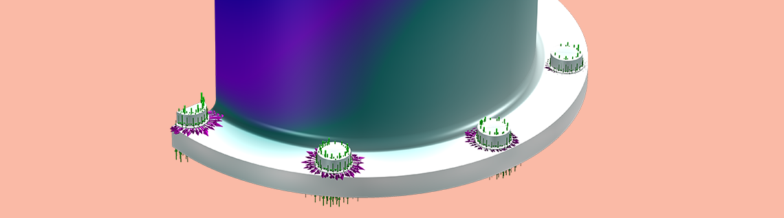
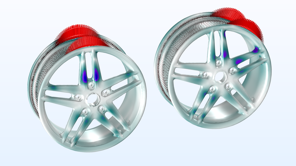
In the load plot groups generated from physics interfaces that live on domains or boundaries (for example, Solid Mechanics or Shell), you will find a disabled plot named Gray Surfaces. By enabling the Gray Surfaces node, you can create a more appealing visualization, as shown below.


Load plot with default settings (left) and after enabling the gray surfaces (right).
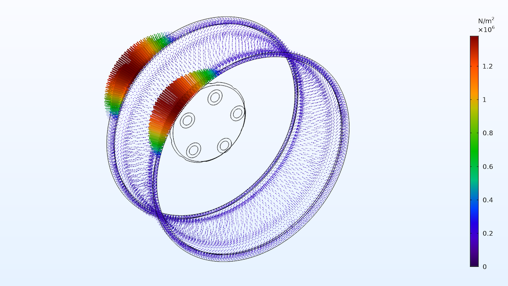
In this example, the load transmitted from the road surface to the rim is, however, less visible when the surfaces are filled. One thing that you can try if the load arrows appear hidden is to modify how the arrows are drawn relative to the boundary. This can be done by changing the Arrow base setting.
![]()
Changing the location of the arrow base.
The same plot as above, after changing the arrows so that the head is placed on the boundary.
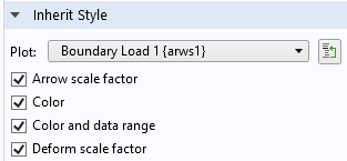
Inheritance of Properties
The first node in each plot group controls a number of properties of the subsequent nodes. This means that you can change important properties for the whole group just by changing the settings in the first node.
The inherited properties.
If you study the settings in the load plots in more detail, each plot actually inherits the properties from its immediate predecessor. This means that if you manually change the settings for a certain node, this change will also apply to all nodes below it within the same plot group.
Arrow Colors
The arrow colors are controlled from a Color Expression subnode under the vector plot.
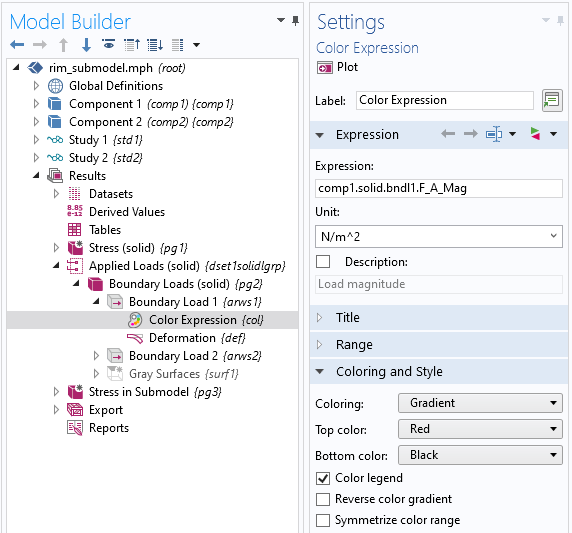
The Color Expression settings.
The default black-to-red gradient scheme is intended to give a rather sober impression. It is, however, not optimal if you really want to read out the values from the legend. By changing Coloring from Gradient to Color table, you will switch to a color scheme with better legibility.
Plotting using the default color table.
Changing the Size and Density of the Arrows
The size of the arrows can be modified in the Coloring and Style section in the settings for the first plot in the plot group. Usually, dragging the slider is a convenient approach for adjusting the arrow size.
Changing the number of arrows requires a bit more consideration. The default is that one arrow is drawn at the centroid of each element (or element face). This may, depending on the actual mesh density, give a visualization that is either too crowded or has too few arrows. In the latter case, the easiest approach is to increase the number in the Gauss-point order text field in the Arrow Positioning section. The arrows are drawn at the Gauss points within the elements or element faces.
As an alternative, you can select Mesh nodes in the Placement drop-down list. In this case, arrows are drawn at the element corners; that is, at the mesh nodes of a first-order element.
Finally, you can select the placement to be Uniform. This is often a good choice if the element size varies considerably over the set of boundaries where the load is active. In this case, the arrows are distributed using an algorithm attempting to make the density of arrows uniform. The arrow density is actually the number you enter divided by the total selected boundary area, not the area where the loads are defined.
![]()
Different types of arrow placement. Upper left: Gauss points, order 1 (the default); Upper right: Gauss points, order 2; Lower left: Mesh nodes; Lower right: Uniform, 200 arrows.
![]()
Same plot settings as above, but the loads are acting on another type of mesh.
If the mesh is very fine, your only option will be, in general, to work with a uniform distribution of arrows.
Displaying a Subset of Load Features
Sometimes, you want to study only the loads generated by a single load feature. Alternatively, you may want to suppress the arrows related to a certain load feature.
This is simple: You just disable the unwanted plots within the plot group. In addition to selecting Disable from the node’s context menu, there are also two handy shortcuts: Select a node, or a number of nodes. Then, press F3 to disable or F4 to enable. (This works for all nodes in the Model Builder tree, not only plots.)
Note, however, that if you disable the first plot in a plot group, it can no longer control the inherited properties. A warning message will be shown. The plotting will, in general, still work satisfactorily, though. If needed, you can remove the inheritance property of the first enabled node, and then do manual changes that also affect the following nodes.
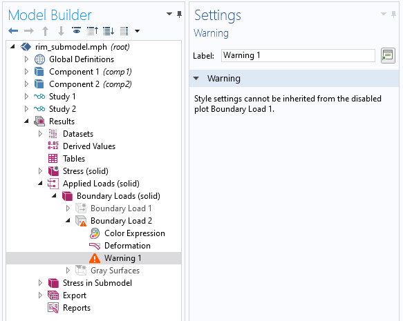
Warning shown if the first plot in a plot group is disabled.
Parametric and Time-Dependent Solutions
The load plots adapt to the currently selected value of time, parameter value, or load case. You can use animations to visualize how the load is varying. If you want to show the loads together with other results, such as stresses, you can just copy-paste the plot nodes into another plot group.
Loads plotted together with stress distribution in the wheel rim for two values of the parameter describing the rotation of the load.
Some Exceptions
Some loads are not applied directly to a geometrical object, but rather at a certain coordinate in space. Examples are loads applied to rigid connectors, rigid domains, and to joints or gears in the Multibody Dynamics interface. Such loads are represented by a Point Trajectories node rather than a vector plot. You can, however, also tune these plots in essentially the same way as described above.
In the Pipe Mechanics interface, the internal pressure load in a pipe is presented as a colored line plot, as it does not have a specific direction. The drag force uses a vector plot, though, since it acts along the pipe.
In the rotordynamics interfaces (Solid Rotor and Beam Rotor), the rotating frame forces are not introduced by adding a load feature; rather, they are inherent in the formulation of the physics interface itself. Load plots are however still created.
Large Deformations
When deformations are large, the question about whether the loads should be displayed on the original or deformed geometry arises. In particular, this is relevant if the forces depend on the deformation.
As a default, the loads are plotted on the undeformed geometry. The plots do, however, come with a Deformation subnode. In most cases, the deformation scale is set to zero. However, if the study is geometrically nonlinear, the scale factor is 1 so that deformations have true scale. By changing the scale factor in the Deformation subnode under the first plot in the plot group, you can create any type of deformation. This is particularly useful if you want to superimpose the loads on, say, a deformed stress plot.
A general remark, valid for all types of plots, is that deformation should only be added when the dataset is represented in the material frame. In the spatial frame, the deformation is already present.
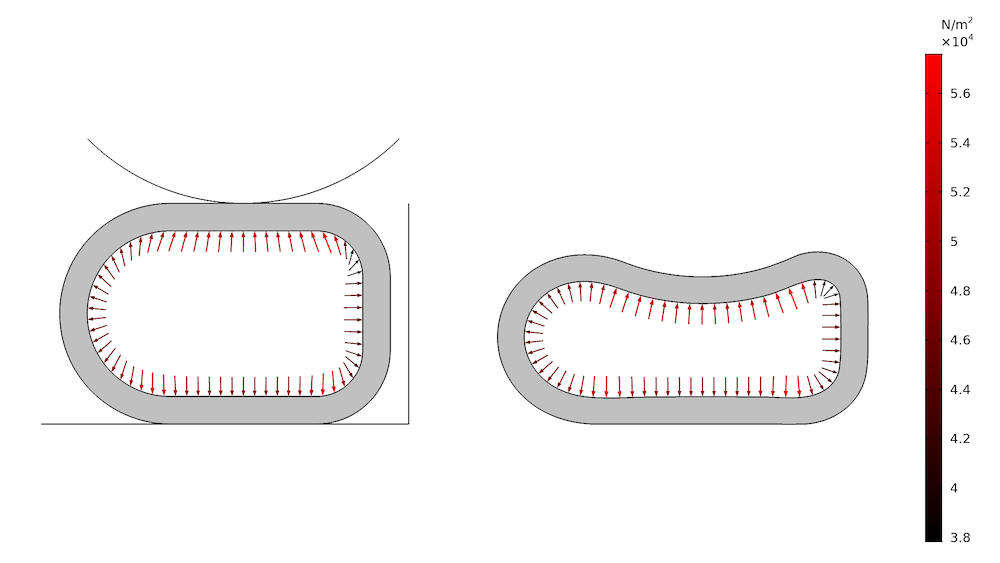
Plotting a pressure load on the deformed and undeformed geometry, respectively.
In the plot above, two things can be noticed. The first is that the arrow directions look strange in the undeformed plot. Loads that change orientation with the solution must be plotted in a deformed configuration in order to make sense.
Secondly, what is actually a constant pressure turns out to have a rather large variation according to the legend. The reason is that the traction is to be interpreted in a “first Piola–Kirchoff” sense. What is shown is the force per original area, but with current orientation. Thus, if a certain loaded area element has become smaller during deformation, the load value shown will also be smaller, since the total load acting on that patch is smaller than if it was not deformed.
Load Visualization During Preprocessing
Often, you want to verify the distribution of the loads for which you just entered an expression. In this situation, you do not yet have a computed solution. Normally, default plots are generated as part of the study being run.


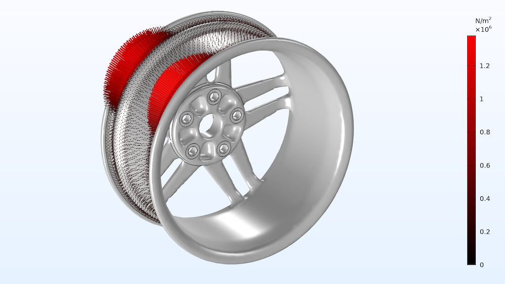
Example of a complicated load expression (this is the tire load on the wheel rim, visualized above).
The key here is that the Get Initial Value operation, which is very fast when compared to actually computing a solution, will generate datasets and default plots for any study in the same way as running the study itself. In order for the Get Initial Value operation to complete successfully, the most important thing is that it is possible to generate a mesh. This does not have to be the mesh that you intend to use when actually solving, but something on which the loads can be plotted must exist. It is possible that you will encounter error messages during Get Initial Value if the input data in general is incomplete or inconsistent (for example, material parameters are missing). Unless it is a really serious problem, the intended datasets and plots will be generated anyway.
It is common that loads are not only a function of space but also time, parameters, or even another solution, for example. What will be plotted is based on the information that the initial values computation has about the model. For example:
- A parameter will take the value given in a Parameters node under Global Definitions, unless the parameter is used for a parametric solution. In that case, the first parameter value in the list is used.
- Loads that are attached to load groups will not be displayed. No specific load group is considered as active during initial values generation. If you want to display such loads, you will have to reassign them temporarily to Active in All Load Groups.
- The time used will be the first time value in the range of times specified in a Time Dependent node.
- If the results are solution dependent, the settings in the Values of Dependent Variables section in the settings for the study will control what you get.
The way default plots work, not only for loads, is that if there already are any plots present for the dataset, then no default plots are generated. This behavior is the same irrespective of whether a full study is run or if only initial values are computed. As an effect, if you change the structure of the load features in any way and want to visualize the new settings, it is not enough to run Get Initial Value again. You should delete the dataset first. This will also remove all plots pointing to the dataset.
As long as you only change the values in existing load features, then it is enough to run Get Initial Value.
Contact Forces
In a contact analysis, the normal contact forces and friction forces will also be available as default plots. The same exact technology used for the load plots is used, so you have the same options for customizing the plots.
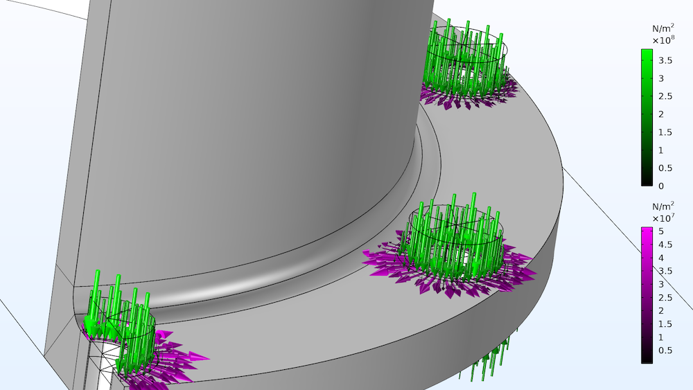
Normal and friction forces as displayed by the default contact force plot.
The Physics Symbols
Even though physics symbols are not directly related to the new load plots, this feature is worth mentioning here and has been available for several versions of the COMSOL® software.
The fact that COMSOL Multiphysics offers a large degree of flexibility in describing loads using, for example, numerical values, parameters, solution-dependent variables, or results from previous studies, comes with a downside in terms of instant visualization. It is not feasible to display the true loads directly when changing a value in the settings for a certain load, and we must resort to the techniques described above.
When working in the physics interface, you have the option of adding physics symbols. The physics symbols show that a certain type of load (or constraint) is present on, say, a boundary. However, it does not show the direction of the load or its amplitude. To include physics symbols in the graphics, you select Enable Physics Symbols in the settings for a physics interface.
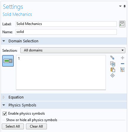
Switching on the physics symbols.
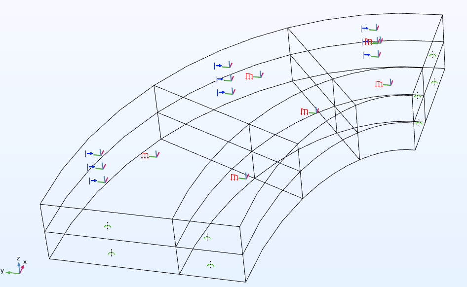
Physics symbols for boundary loads, prescribed displacements, and symmetry conditions are shown in this figure.
To enhance the visualization of physics symbols, any node that can generate a physics symbol also has an individual control for whether the symbols are active or not. This is particularly useful for boundary conditions in which many geometrical entities are selected, since one physics symbol is shown per selected entity.
Controlling the display of physics symbols for an individual boundary condition. This section is only visible when physics symbols are activated for the physics interface as such.
Concluding Remarks
The load plots available in COMSOL Multiphysics are used in many of the structural mechanics models available in Application Libraries and Application Gallery. Take a look at the example models discussed in this blog post:
- Submodel of a Wheel Rim
- Thick Plate Stress Analysis
- Hyperelastic Seal
- Prestressed Bolts in a Tube Connection
- Pratt Truss Bridge
Contact us if you have any questions about how this postprocessing functionality can benefit your structural analyses:

Comments (1)
Jay Puckett
December 9, 2019Nice new feature, overdue. Well written post. Thank you. jp