

Overhead power cables can be seen almost everywhere in the United States, but there are also many underground power cables that we can’t see. They have the advantage of protection from wind and snow damage and, due to their shielding, have greatly reduced electromagnetic field emission. One disadvantage of underground cables is that they heat up significantly, which leads to degradation of the insulation and failure. Let’s see how to model electromagnetic heating in the COMSOL Multiphysics® software.
Properties of Underground Power Cables
A typical underground three-phase electrical cable is made up of a bundle of three conductive cables. Each individual cable is stranded, meaning it is composed of many wires that are twisted together and compressed so that the strands are in good electrical contact. The cable can also have shielding such as a metal foil. A polymer material between the cable and shielding provides electrical insulation. Wound paper, fluids, and even pressurized gases are also used as electric insulators. The entire insulated cable bundle is then encapsulated within another dielectric and a metal sheath as well as an outer polymer coating, which protects the cable from the environment.


Left: An underground three-phase electrical cable. Right: Cross-sectional schematic of a buried three-phase cable.
The alternating current passing through the cable results in a time-varying magnetic field, which causes induced currents in the cable as well as in the surrounding metal sheaths and foil. The currents lead to a combination of Joule heating and induction heating. The cable bundle then begins to heat up, possibly causing it to fail, hence our interest in building a predictive computational model.
The electrical analysis of the cable is fairly straightforward. We usually know all of the relevant material properties (electric conductivity, permeability, and permittivity) in the cable bundle as well as exactly how much current flows through the cable and at what frequency. However, we only have a rough understanding of the electrical properties of the surrounding soil.
Thermally speaking, there are even more unknowns. The thermal properties of the surrounding soil vary based on its composition and moisture content. Even within the cable, although we know the material properties, there can be thin layers of material and small air gaps that significantly change the peak temperature.
Let’s find out how we can model these types of cables using COMSOL Multiphysics.
Modeling Electromagnetic Fields in an Underground Cable
We can reasonably assume that underground cables are long and the surrounding environment is relatively uniform. These assumptions allow us to simplify our model by considering a 2D cross-sectional slice, similar to the one shown in the schematic above. We know that the three-phase current in the cables varies at a fixed frequency. We also know the maximum current.
We assume that the stranded bundle of copper wires is compressed together with good electrical contact, so we treat each of the three copper cables as one uniform domain across which the current can redistribute itself. Thus, we use three different Coil features to excite the three copper cables, as shown in the screenshot below. The applied excitation is of the form: 1[kA]*exp(-i*120[deg]).
That is, a 1kA peak current flows through the three cables, but the relative phases are shifted by 120° between each.
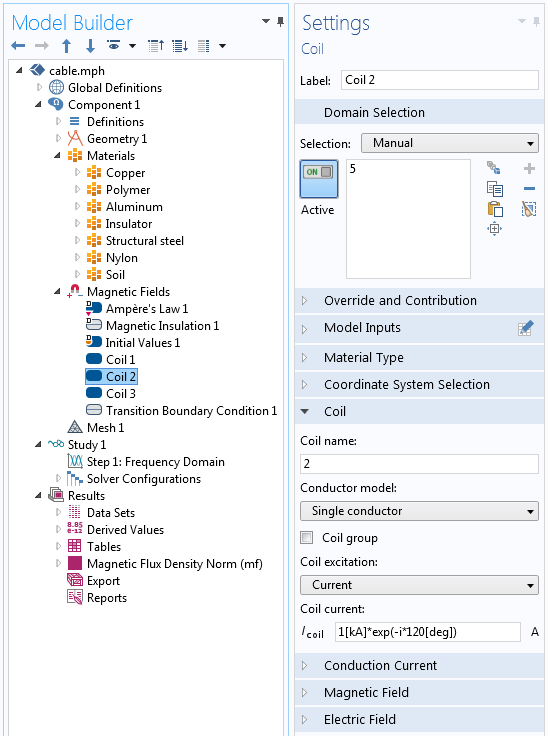
The Coil feature sets up the current flowing through one of the cables. The other two cables carry the same current, but with a 120° phase shift.
Next, we consider the thin layer of metal shielding. If the thickness of this layer is small compared to the other dimensions, then we model this metal layer via the Transition boundary condition, as shown below. This boundary condition allows us to enter a thickness and specify a set of material properties at an internal boundary of the model. The advantage of this condition is that we don’t need to explicitly model the geometry and thus don’t need to mesh this thin layer of material.
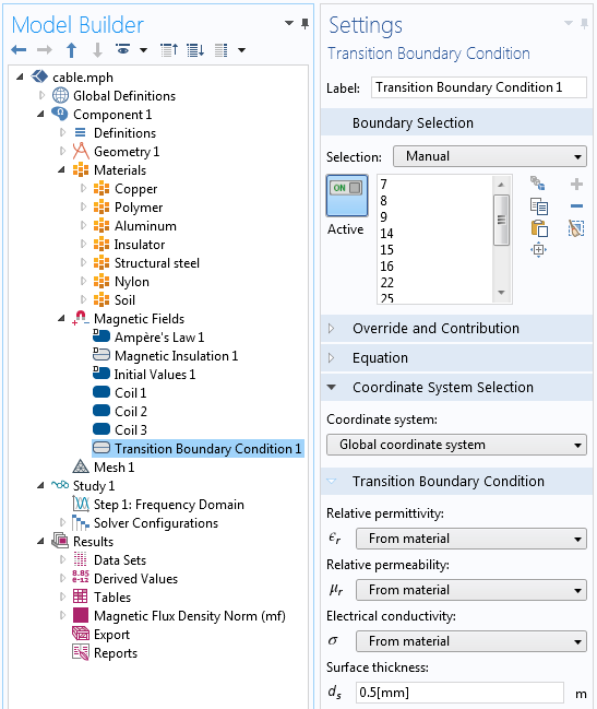
The Transition boundary condition in which the layer thickness and material properties can be entered.
The magnetic fields can extend some distance outside of the cable. Since we want to know how quickly the fields drop off, we model a region of soil around the cable. We choose this region’s size by studying progressively larger domains until the field solution shows minimal variation with an increasing domain size, a procedure described in an earlier blog post on choosing boundary conditions for coil modeling. The results of such an analysis, seen in the image below, show the magnetic field and cycle-averaged losses. It is these losses that lead to a rise in temperature.
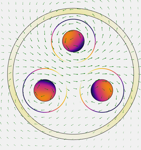
The losses in the cable bundle and shielding with arrows representing the magnetic field. The arrow lengths are logarithmically scaled relative to the magnetic field strength.
Predicting the Temperature Rise in COMSOL Multiphysics®
Modeling the temperature rise of the cable seems relatively straightforward — we simply take the computed losses and include them in a thermal model. We add the Heat Transfer in Solids physics interface to our model and, within the Multiphysics branch, use the predefined features to set up a bidirectional coupling between the electromagnetic and thermal problem. Either the Frequency-Stationary or Frequency-Transient study type can be used to solve the electromagnetic problem in the frequency domain while solving the thermal problem in the steady state or time domain.
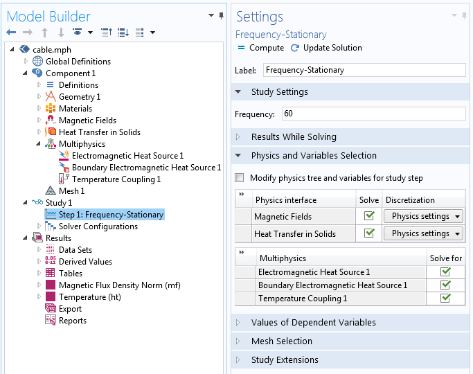
The Frequency-Stationary solver and multiphysics settings for creating the bidirectionally coupled electromagnetic heating model.
Using the Thin Layer Boundary Condition
Now, even though the thermal model appears straightforward, there are a number of things that we need to keep in mind as well as features of the software that we want to be aware of. For one, the cable bundle has several thin layers of material, such as the shielding and coatings, that we might not want to model explicitly. For these, we use the Thin Layer boundary condition, which has the option of modeling the thin layer as a Thermally thin approximation, Thermally thick approximation, or General layer, as shown in the screenshot below.
The Thermally thin approximation is appropriate when the material layers have a relatively much-higher thermal conductance than their surroundings, whereas using the Thermally thick approximation is better for material layers with a relatively much-lower conductance. The General type should be used for any intermediate cases, where there are significant thermal gradients both normal to and tangentially along the layer of material. All of these options allow you to specify the layer thickness and properties, and the General type additionally allows you to specify a composite of up to five different layers.
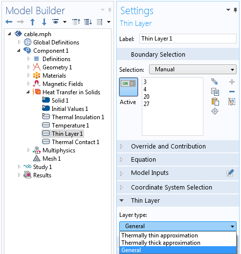
The Thin Layer boundary condition.
The Thin Layer boundary condition is appropriate for well-defined layers of material, with known thicknesses and properties. We also need to consider the thermal resistance that arises when two materials are in contact. Heat transfer between rough surfaces in contact occurs when there is:
- Conductive heat transfer due to the solid materials being pushed together
- Conductive heat transfer through the thin layer of air
- Radiative heat transfer between the exposed surfaces
These effects can all be modeled via the Thermal Contact feature, seen in the following screenshot.
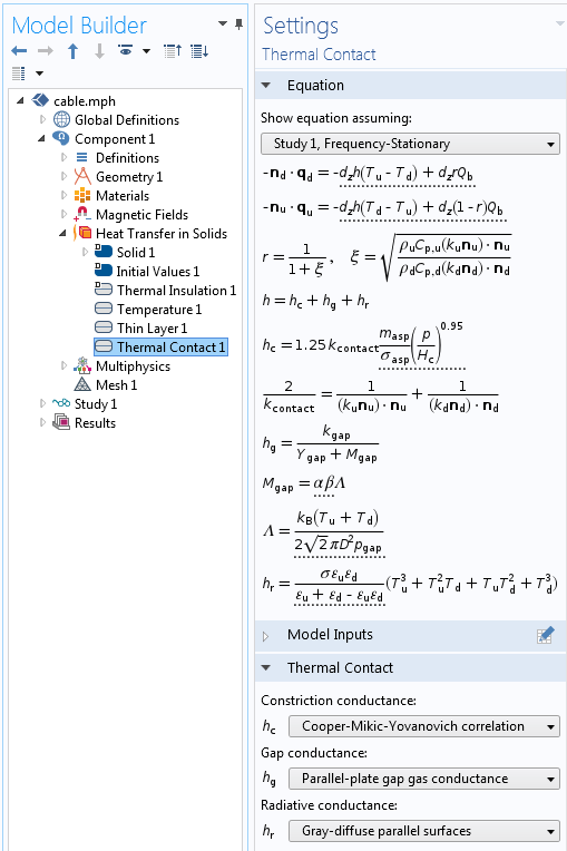
The Thermal Contact feature and equations.
The conductive heat transfer through the solids is strongly affected by the contact pressure. This pressure can be computed from (and coupled with) a structural analysis, as exemplified by these tutorial models:
Modeling the Thermal Environment and Domain
Next, we need to consider the thermal environment, which has a great deal of variability that directly affects the cable temperature. The surrounding soil, concrete, and rocks have thermal conductivities that range from 0.1 to 5 W/m/K and densities that range from just over 1000 kg/m3 for very loosely packed soil to over 3000 kg/m3 for solid rocks. Their specific heat capacities also vary from ~500 to 1500 J/kg/K. Furthermore, these values do not remain constant. For example, the thermal conductivity of dry and wet sand can differ by over an order of magnitude: from ~0.2 to 4 W/m/K. It is also helpful to introduce the thermal diffusivity, which is defined as \alpha = \frac{k}{\rho C_p} and ranges from roughly 10^{-8} -10^{-5} m^2/s for these materials.
In addition to the huge variability of the soil’s thermal properties, the thermal boundary conditions at the surface are rarely well defined. There is both convective cooling to the air and radiative cooling to the sky. The magnitude of this cooling is greatly affected by the local and temporary features at the surface. For example, dead leaves or loosely packed snow can act as a very good layer of thermal insulation that is difficult to quantify with any precision.
Lucky for us, the cables are buried deep enough that these temporary variations at the surface can often be neglected. Thus, it is reasonable to approximate the heat balance at the surface with a combination of three boundary conditions:
- A Heat Flux boundary condition representing the solar heat load based on the latitude and time of year
- Another Heat Flux boundary condition representing the convective cooling to the average ambient air temperature
- A Diffuse Surface boundary condition representing the radiative cooling to the effective sky temperature
The solar heat load and ambient air temperature can be entered approximately or from the American Society of Heating, Refrigerating, and Air-Conditioning Engineers database of weather station data, as we describe in a previous blog post. The effective sky temperature ranges from about 230 K to 285 K (-45°C to 10°C), depending on the air temperature and cloud cover, with a typical ground surface emissivity of 0.8–0.95.
We must also consider the width and depth of our thermal domain. We need to model a sufficiently large domain of soil such that the boundary conditions don’t affect the results. For thermal loads that vary sinusoidally in time with cycle period \tau, the distance D from the boundary at which the temperature oscillation is reduced by approximately 90% relative to the oscillation at the surface is given by: D = \sqrt{\frac{\tau \alpha}{2 \pi}}.
Assuming that the thermal boundary conditions vary sinusoidally over the year, and assuming a very high thermal diffusivity, a good rule of thumb is to model a domain that extends at least eight meters beneath the surface and is at least three times the burial depth on either side, with thermal insulation boundary conditions on the vertical boundaries and a fixed temperature boundary condition at the bottom boundary. A Temperature boundary condition is used to fix the temperature at the bottom to the average of the surface temperature over an entire year. This is a good approximation of the large thermal mass of the ground.
We can also investigate a larger soil domain to see if peak temperatures are noticeably affected. Of course, if there are known subsurface features, such as nearby water mains or building foundations, these should be included in the model.
Solving the Model
We can solve the model using either a Frequency-Stationary or Frequency-Transient study type. Both solve for the frequency-domain form of Maxwell’s equations, but solve the thermal model as either a steady-state or time-dependent problem. Solving for the steady-state temperature requires a bit of care in interpreting the results. A steady-state analysis will assume that all thermal transients have died out, a rather severe assumption. Such results must be interpreted with care. Solving the transient problem, on the other hand, can consider all of the changing environmental conditions and loads and will give not just the peak temperatures but also the duration at which different materials are at different temperatures.
The screenshot below shows a typical model setup and sample results.
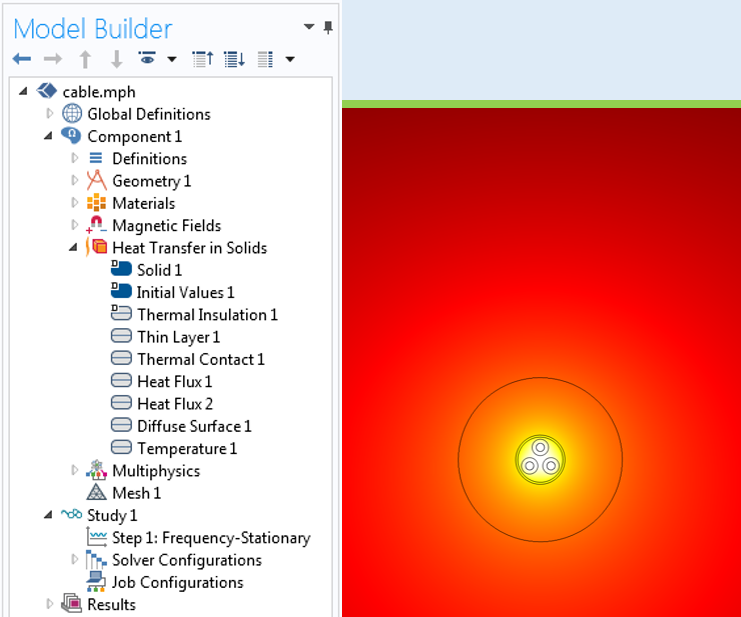
The thermal model and representative results of the cable’s temperature. The magnetic fields are only solved for the smaller circular domain around the cable, since the magnetic fields drop off rapidly in intensity.
Closing Remarks on Modeling the Electromagnetic Heating of Underground Cables
Here, we have shown the appropriate COMSOL® software features and modeling approaches for computing the temperature rise in underground power cables. When solving such problems, keep in mind the variability in the solution that can be introduced due to the changing thermal environment, imprecisely known soil properties, and even small air gaps or standoffs within the cable itself. Of course, COMSOL Multiphysics (along with the AC/DC and Heat Transfer modules) is a great tool for modeling these situations and for considering all of the variability in the model inputs.
Interested in using COMSOL Multiphysics to model electromagnetic heating?
Further Reading
- Learn more about electromagnetic simulation on the COMSOL Blog:
- Download the Cable Tutorial Series, which features six tutorial models and related documentation

Comments (7)
M. ELADAWY
February 23, 2017Very attractive study
can you send this mph file to be a reference study for all who are concerned with heating of underground cables?
Thanks
Walter Frei
February 27, 2017 COMSOL EmployeeHello,
This blog isn’t really meant to present a reference study, but rather, it is meant to highlight the following modeling features:
– Coil Domains with current excitation at different phases
– Transition boundary condition
– General Thin Layer thermal boundary condition
– Thermal Contact boundary condition
and to highlight how these features are useful for this type of modeling.
The discussion at the end is also meant to introduce some of the complexity in correctly modeling the thermal environment.
Shatha Al-Doori
February 18, 2021Hello Walter
I am working with modeling three physics together EM ,Heat Transfer and Laminer flow, and I am sure about all the conditions, but still I have some difficulties that makes error
Bin Sun
March 11, 2017Can you tell me the detail information of your soil? like the relative permittivity and permeability? Is that possible to share the mph file? I am not familiar with the heating transformer part. Thanks a lot.
Walter Frei
March 13, 2017 COMSOL EmployeeHello Bin,
The relative permittivity and permeability and conductivity of the soil have significant variability (just as the thermal properties do.) Especially the permittivity and conductivity are highly dependent upon water content. We do not attempt to tabulate these properties here, as there are many handbooks and databases of such properties available. Always keep in mind, though, that significant variability exists in any real-world situation.
gomaa osman
May 31, 2017Hello Walter,
I am working in heat transfer of underground cable, i need to make the thermal conductivity of the soil change with temperature of the cable surface (i have the equation), but how can take the temperature of the cable surface to this equation
OR how can take the temperature at any point in the model or at any layer of the cable and the soil as variable to any equation
thanks
Caty Fairclough
June 21, 2017Hi Gomaa,
Thanks for your comment!
For your questions, please contact our Support team.
Online Support Center: https://www.comsol.com/support
Email: support@comsol.com