How to Model Rotating Machinery in 3D

Electrical machines are an important pillar in modern industrial society. Among the different types of electrical machines, rotating machines such as generators and motors take up a central role. The Rotating Machinery, Magnetic physics interface in COMSOL Multiphysics is designed specifically for modeling these systems. Follow along as we explore how to model rotating machinery and detail best practices for working with this feature.

The Geometry of a Rotating Machine

In any rotating magnetic machine, there are two parts: the stator and the rotor, separated by an air gap enabling the rotor’s rotation. The Rotating Machinery, Magnetic interface uses the moving mesh approach to model this rotation, as the finite element method does not support rotations.

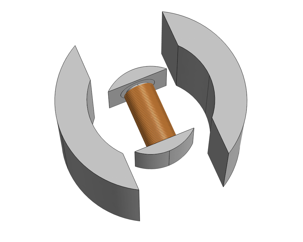
Geometry of a DC commutated motor that includes two permanent magnets and a rotating winding.

The machine’s geometry is cut (usually along the air gap) into two parts: one containing the stator, and one containing the rotor. The two parts are then meshed separately. During simulation, the part containing the stator remains stationary while the part containing the rotor moves. The two parts with the corresponding meshes are always in contact at the cut boundary.

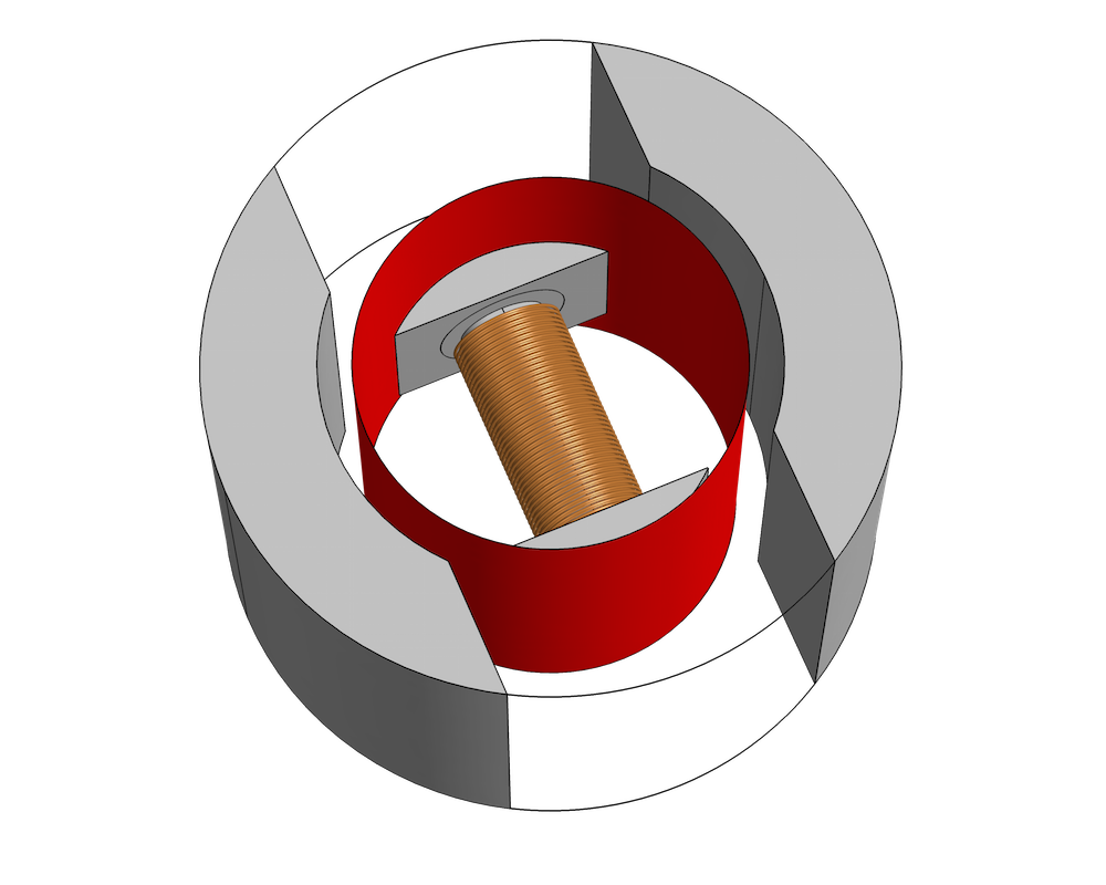
The geometry must include the air region between the magnets. Red represents a possible choice for the cut boundary.

By default, the last step in a geometry sequence is to finalize by forming a union, uniting all of the geometrical objects and meshing them as a single object. To mesh the two parts separately, the objects must be finalized by forming an assembly. Using unions and other operations, create a single geometry object for the stationary part and another one for the rotating part. Then, choose Form Assembly in the finalization node of the geometry sequence. During finalization, an identity pair is automatically created under Definitions, identifying the common (contacting) boundaries of the two objects.

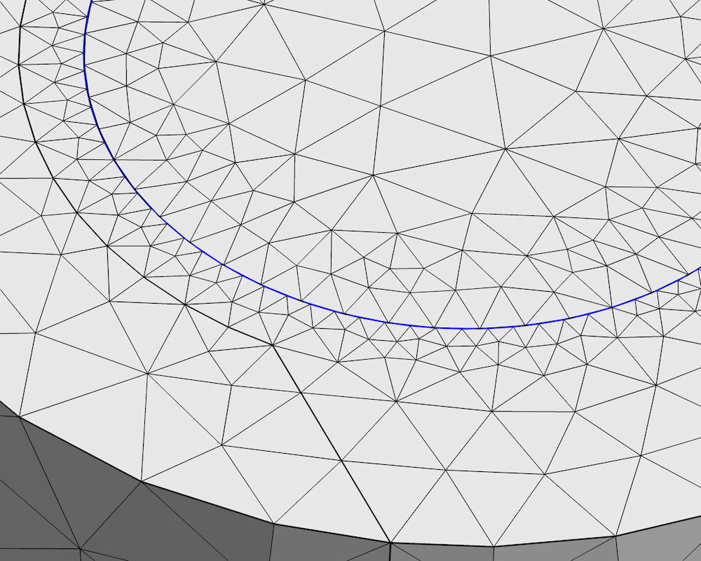
A close-up of the DC motor’s mesh. The rotating and stationary parts are meshed separately, as indicated by the different positions of the mesh nodes on the two sides. The boundaries highlighted in blue are collected in an identity pair. During rotation, the meshes slide on each other, remaining in contact at the pair.

Watch a video to learn more about using Form Assembly in rotating machinery models.

We can now define the dynamics of the system using the Rotating Machinery, Magnetic interface. Use the Prescribed Rotation feature to specify an angle of rotation (which can be time dependent) or the Prescribed Rotational Velocity feature to enter a constant angular velocity. After applying one of these features, the COMSOL Multiphysics software will enable moving mesh for the selected domains and the set-up of the appropriate transformations of the electromagnetic field.

The Prescribed Rotation or Prescribed Rotational Velocity features must be applied to the rotating part containing the rotor.

What happens at the cut? Physically, the electromagnetic field is continuous in the air gap, assuming a homogeneous material. In contrast to other interior boundaries, continuity of the fields is not automatically imposed across the pair. To enforce this condition, use the Continuity pair feature on the identity pair.

The Mixed Formulation

The Rotating Machinery, Magnetic interface solves Maxwell’s equations to compute the distribution of the electromagnetic field. Most quantities of interest (e.g., the applied torque) can be computed once the fields are known. In time-dependent analyses, the interface applies the quasistatic approximation, which neglects the displacement current density, or equivalently assumes that capacitive effects in the machine are negligible. With this approximation, all of the currents in the machine are either externally applied (i.e., through an excited winding) or are eddy currents induced in the machine’s conductive parts. The nonconductive parts, like the air gap, do not carry any current density.

There are two approaches used in this interface to solve Maxwell’s equations: the vector potential formulation and the scalar potential formulation. In the former approach, a vector field, \mathbf{A} (the magnetic vector potential), is introduced and the approach defines the magnetic flux density and the electric field as

With these definitions, the \mathbf{B} and \mathbf{E} fields automatically fulfill two of Maxwell’s equations: Faraday’s law and the magnetic flux conservation law (or magnetic Gauss’ law). These are written as such:

The equation to be solved is Ampère’s law:

The vector potential formulation is used in the Magnetic Fields physics interface.

The scalar potential formulation is only applicable in regions where the electric current density is zero. In this case, a scalar field V_\textrm{m} (the magnetic scalar potential, not to be confused with the electric potential) is introduced and the magnetic field is defined by the approach as the gradient of this potential. With this definition, Ampère’s law is automatically fulfilled and the magnetic flux conservation law is solved. This formulation is used in the Magnetic Fields, No Currents physics interface.

Compared to the vector potential formulation, the scalar potential formulation introduces fewer degrees of freedom and leads to an “easier” problem to solve. The downside is, of course, that it can only be used in the absence of currents. Normally, this condition would restrict the applicability to special cases, like stationary studies of permanent magnets. But, thanks to the quasistatic approximation, this formulation can also be applied to nonconductive regions in time-dependent analyses.

In the case of 3D models, the scalar potential approach offers another important advantage. When used with a pair feature such as the Continuity feature, this formulation ensures a more accurate coupling of the magnetic flux density — a quantity that is central within the modeling of magnetic machines.

These two formulations can also be used together by combining the vector potential formulation for conductive or current-carrying domains and the scalar potential formulation for the air gap and nonconductive domains. Referred to as mixed formulation, this approach is particularly useful in 3D models due to an increased accuracy of the pair coupling given by the scalar formulation. In 2D models, for in-plane magnetic fields, the discretization scheme used for the vector potential is similar to that used for the scalar potential. Thus, in 2D in-plane cases, using the mixed formulation is not necessary.

By default, the Rotating Machinery, Magnetic interface applies the Ampère’s Law feature (that is, the vector potential formulation) to all domains, as it is the most general formulation. Apply the Magnetic Flux Conservation feature (which implements the scalar potential formulation) to the current-free domains, such as the air gap and other nonconductive regions, overwriting Ampère’s Law. The appropriate conditions will be imposed at the interface between the scalar and the vector potential regions using the Mixed Formulation Boundary feature. Note that the Continuity pair feature couples the dependent variables on the two sides of the pair, so make sure that the same formulation is used on either side. For improved numerical stability, a Gauge Fixing for A-Field feature can be applied on all of the vector potential domains, as is often done in the Magnetic Fields interface.

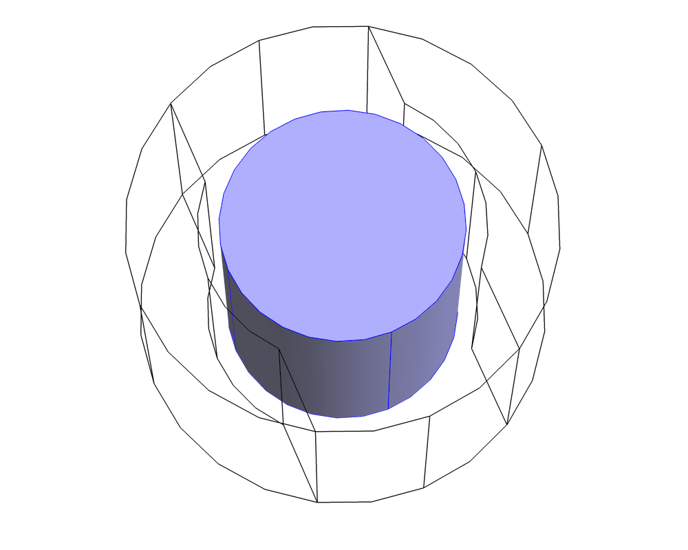
The Ampère’s Law feature is applied only to the inner portion of the rotating part, where there is a current-carrying winding. Note that the selected region is smaller than the entire rotating part, which extends to the cut boundary. For increased accuracy, the scalar potential formulation should be used near the pair condition.

Using the mixed formulation is quite simple and straightforward, but keep in mind the mathematical background of the formulations and its limitations. The most important condition on the applicability, the one that is most prone to causing errors, is that the scalar potential can only represent an irrotational (curl free) magnetic field. In practice, there cannot be closed curves in the scalar potential region that completely enclose (“chain”) a current.

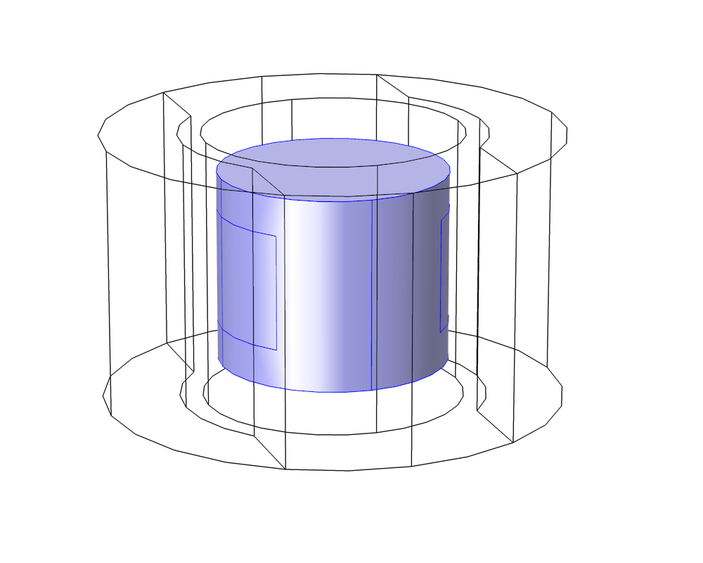
The reason for this condition derives from the definition of the scalar potential and from Maxwell’s equations. In regions where the scalar potential formulation is used, the integral of the magnetic field along a closed curve is always zero, since the field is the gradient of the potential. At the same time, from Ampère’s law, we know that the integral of the magnetic field along a closed curve must be equal to the total current chained by the curve. Consequently, there is no solution (no possible configuration of the potential) unless the chained current is exactly zero. If we try to solve a problem that does not respect this condition in COMSOL Multiphysics, the solver will not converge. The figure below illustrates this concept, where vector potential regions are represented in blue and scalar potential regions are bounded in gray.

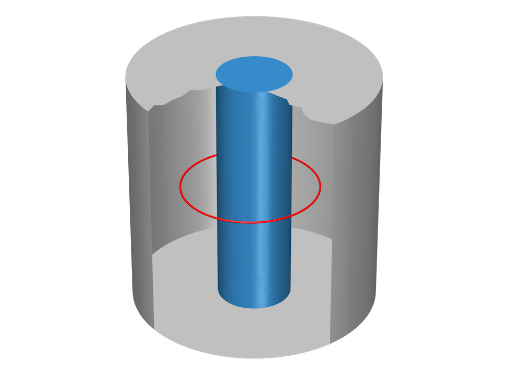
A closed curve in the scalar potential region “chains” a vector potential region that can carry a current (the current return path is on the outside of the geometry). This model may not have a solution.

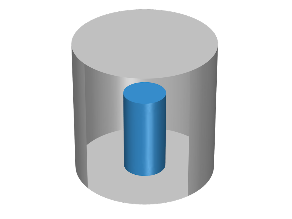
The figures below represent valid geometries in which scalar potential regions are simply connected, meaning that they do not have vector potential “holes” going all the way through.

Relative Motion and Frames

In a rotating machine, the relative motion of the stator and rotor is central to the machine’s operation. Electromagnetic problems involving bodies in relative motion are not trivial — in fact, over a hundred years ago, questions about this topic sparked the development of the theory of relativity.

Typically, the first step in solving such a problem is to select a frame to use when formulating equations. A frame is simply a choice of a coordinate system and axes for each point in space. A natural choice is to select a fixed Cartesian coordinate system, sometimes called the “laboratory” frame and referred to as the spatial frame in COMSOL Multiphysics. In this frame, the stationary part is fixed while the rotating part moves.

Another possible choice is to apply a Cartesian coordinate system at each point in space, as done for the spatial frame, but then let the coordinate system follow the movement of the point as it rotates. In this frame, the material constituting the machine is always stationary (the frame itself moves with it), so the frame is called the material frame. In the stationary part of the machine, the spatial and material frames coincide, since there is no movement. Meanwhile, in the rotating part, the material frame rotates with respect to the spatial frame. Both of these frame choices are equivalent in the sense that they provide the same results, as long as the proper transformations are applied.

By default, the coordinates of the material frame are uppercase letters (X, Y, Z), while the coordinates of the spatial frame are lowercase (x, y, z). The names of the coordinates denote the components of a vector in a certain frame; for example, the electric field components are Ex, Ey, Ez in the spatial frame and EX, EY, EZ in the material frame.

The problem is automatically formulated and solved by the physics in the material frame. For postprocessing, it is often interesting to look at the variables and fields in the spatial frame, as these are quantities seen by an observer at rest with respect to the stator. For this reason, the physics automatically transforms and defines all of the vector fields in the spatial frame. Spatial and material variables are identified in the expression list by the frame in parentheses, as shown in the figure below.

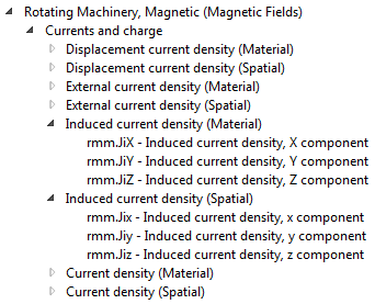
Vector quantities are defined with components in both the spatial frame and the material frame.

Most vector quantities are merely rotated when transformed from the material to the spatial frame, and their norms are invariant. An important exception occurs for the electromagnetic field, particularly the electric field, which transforms according to the Lorentz transformation rules. For nonrelativistic velocities, the fields in the two frames are related by the equations

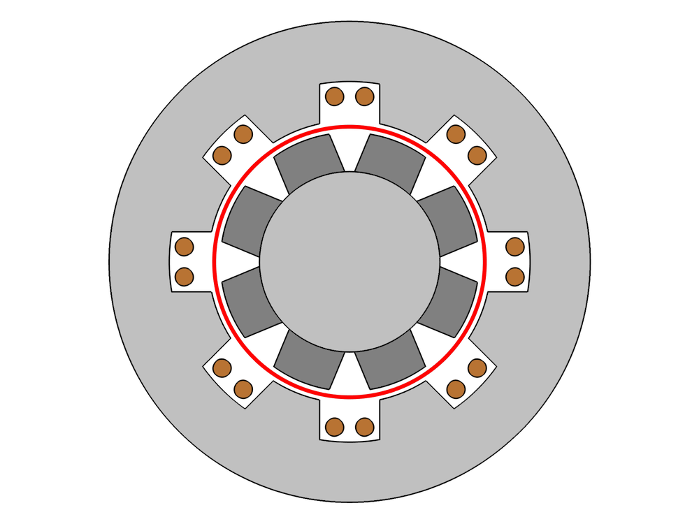
Let’s begin by looking at the geometry of a 2D generator. In the figure below, the red line indicates the separation between the rotating and the stationary parts. The darker domains depict the permanent magnets in the rotor, while lighter domains indicate iron that can be saturated, and the copper domains represent the generator’s windings. The white region identifies air.

The electric field in the material frame is the field “seen” by the conductive material, driving the current density. In general, it is different from the electric field in the spatial frame, as illustrated below.

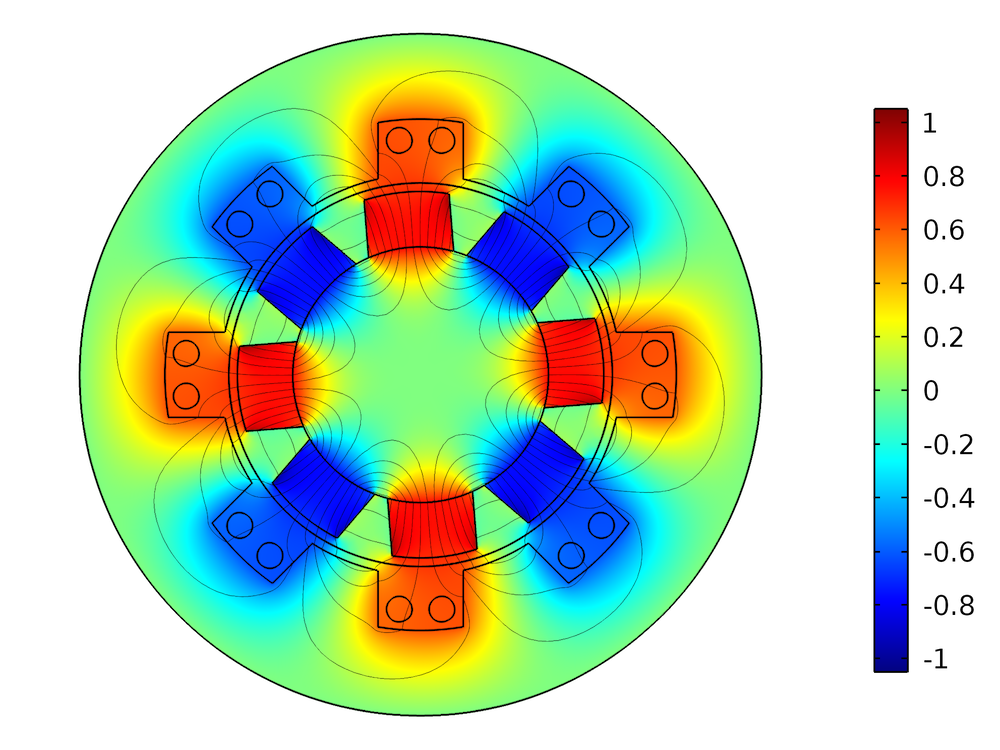
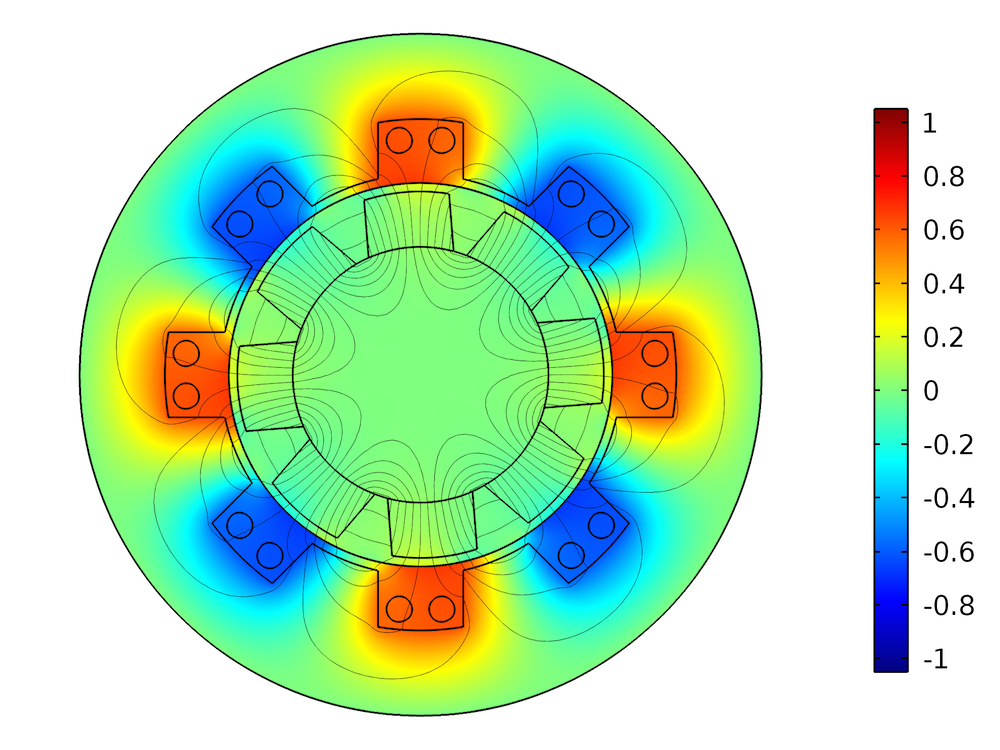
Left: The out-of-plane component of the electric field in the spatial frame during the rotation (in V/m). The magnets in the rotor move with respect to an observer in the laboratory frame, so there is an induced electric field. Right: The out-of-plane component of the electric field in the material frame (in V/m). Because the magnets are stationary in the rotating part’s frame, there is no significant induced electric field. The electric field in the stationary part is the same in the material frame and the spatial frame.

Setting Up the Solvers

The solver set-up must be tailored to the desired simulation. A Stationary study can be used to model the rotating machine’s behavior in stationary conditions in which the rotor is fixed and transient effects have decayed. Instead, a Time Dependent step can be used to study what happens during rotation.

When using the Time Dependent step, it is important to specify the correct initial values that correspond to the physical situation under investigation. If this is the first step in the study, the initial values for the fields are taken from the Initial Value feature (by default, zero). Alternatively, a Stationary step can be solved before the Time Dependent step in order to provide a nonzero initial value for the transient simulation.

In general, a Stationary step is added if excitations are “already active” (e.g., the permanent magnets in the generator), as opposed to excitations that are “turned on” at the beginning of the transient analysis. In models featuring both forms of excitation, like the DC commuted motor, it is important to disable the features responsible for the transient excitation in the Stationary step — that is, if the simulation is designed to model behavior when the transient excitation is “turned on”.

Summary

An advanced topic by nature, the modeling of rotating machinery can be quite challenging. Here, we have presented some of the concepts involved in the modeling of a rotating magnetic machine as well as the procedures and best practices to follow when working within this interesting application. The Rotating Machinery, Magnetic interface and the Magnetic Fields interface, which constitutes the core of the functionality, are powerful tools for analyzing and optimizing these intricate systems.

In a future blog post, we will explore the role of sector symmetry, in addition to these techniques, in modeling rotating machinery in 3D. Stay tuned!

Further Steps

• Download these tutorial models to try it yourself:
  • Generator in 2D
  • Rotating Machinery in 3D

Editor’s note: We published a follow-up blog post on this topic on 2/18/16. Read about the key concepts behind modeling 3D rotating machines here.