Say you are working on a modeling case where loads are moving in such a way that they cross over different mesh elements and boundaries during the simulation. In these cases, among other instances, you may want to apply a boundary condition to only part of the geometrical boundary or only under certain conditions. In this blog post, we’ll discuss how you can utilize the flexibility of COMSOL Multiphysics to handle such situations.
Categorizing Boundary Conditions
In the mathematical treatment of partial differential equations, you will encounter boundary conditions of the Dirichlet, Neumann, and Robin types. With a Dirichlet condition, you prescribe the variable for which you are solving. A Neumann condition, meanwhile, is used to prescribe a flux, that is, a gradient of the dependent variable. A Robin condition is a mixture of the two previous boundary condition types, where a relation between the variable and its gradient is prescribed.
The following table features some examples from various physics fields that show the corresponding physical interpretation.
| Physics | Dirichlet | Neumann | Robin |
|---|---|---|---|
| Solid Mechanics | Displacement | Traction (stress) | Spring |
| Heat Transfer | Temperature | Heat flux | Convection |
| Pressure Acoustics | Acoustic pressure | Normal acceleration | Impedance |
| Electric Currents | Fixed potential | Fixed current | Impedance |
Within the context of the finite element method, these types of boundary conditions will have different influences on the structure of the problem that is being solved.
Neumann Conditions
The Neumann conditions are “loads” and appear in the right-hand side of the system of equations. In COMSOL Multiphysics, you can see them as weak contributions in the Equation View. As the Neumann conditions are purely additive contributions to the right-hand side, they can contain any function of variables: time, coordinates, or parameter values.
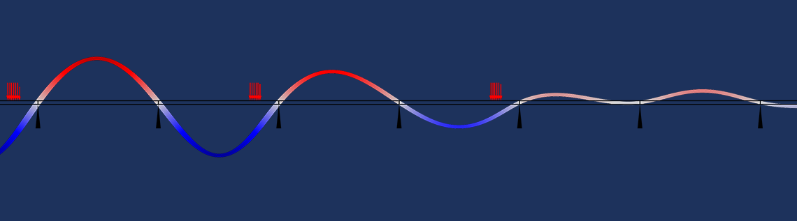
Let’s consider a heat transfer problem where a circular heat source with a radius R is traveling in the x direction with a velocity v. Its intensity has a parabolic distribution with a peak value q_0. A mathematical description of this load could be
For a traveling load, it is obviously not possible to have domain boundaries, or even a mesh, that fits the load distribution at all times.
The load distribution itself can be entered in a straightforward manner. Since the variable for the radial coordinate, r, will be used in two places, it is a good idea to define it as a variable. The entire input for the moving heat source is shown below.
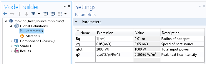
Parameters describing the moving heat source.
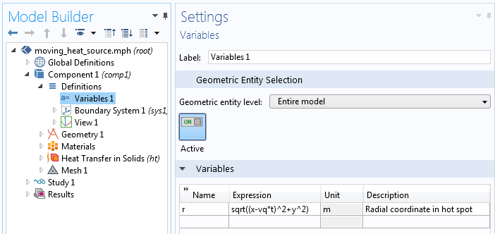
The variable describing the local radial coordinate from the current center of the traveling heat source.
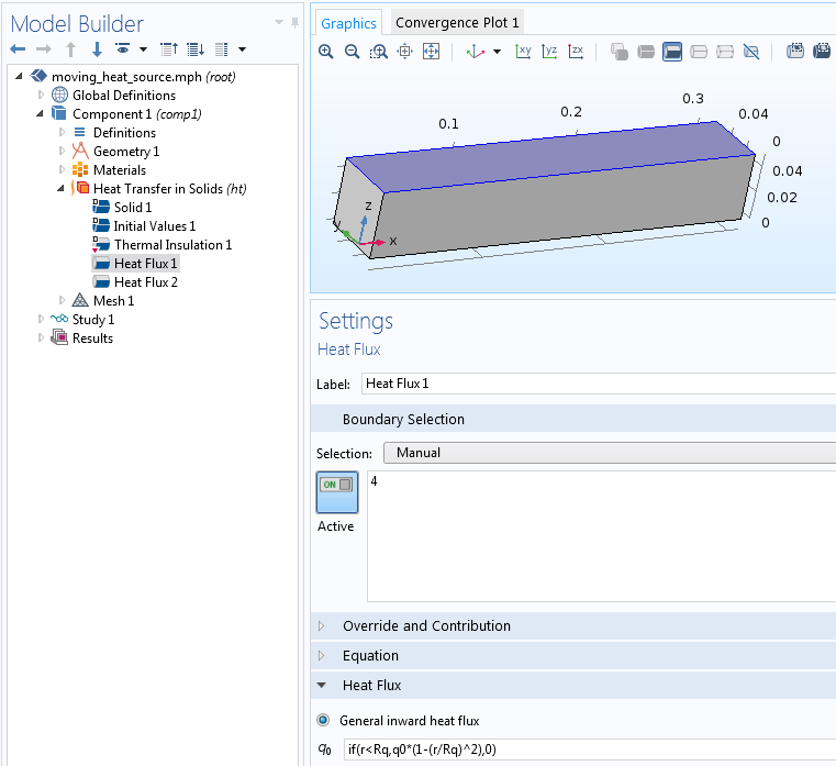
Input of the heat flux.
The results from a time-dependent simulation using such data are depicted in the following animation. Symmetry is assumed in the yz-plane, so the load is actually applied on a moving semicircle.
Animation of the temperature distribution as the heat source travels along the bar.
Dirichlet Conditions
Where a Dirichlet condition is given, the dependent variable is prescribed, so there is no need to solve for it. Equations for such degrees of freedom can thus be eliminated from the problem. Dirichlet conditions therefore change the structure of the stiffness matrix. When looking in the Equation View of COMSOL Multiphysics, these conditions will appear as constraints.
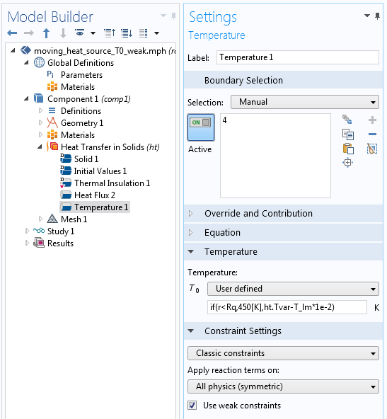
Assume that you want the traveling spot to prescribe the temperature as exactly 450 K. This may be a bit artificial, but it displays an important difference between the Neumann condition and the Dirichlet condition. If you were to add a Temperature node and enter a similar expression ( if(r < R,450[K],0)), it would mean setting the temperature to absolute zero on the part of the boundary that is not covered by the hot spot.
The intention is, however, to switch off the Dirichlet condition outside of the hot spot. There’s a small trick for doing so. If you instead enter if(r < R,450[K],ht.Tvar) as the prescribed value, you will get the intended behavior (shown in the following animation).
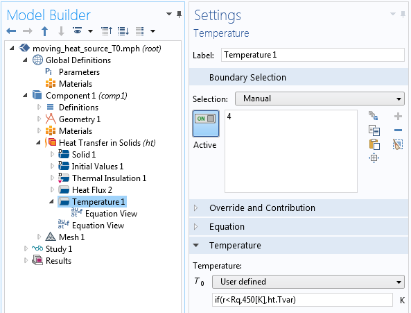
Settings for a conditional Dirichlet condition.
Animation of the temperature distribution as the prescribed temperature spot travels along the bar.
In order to understand how this works, enable the Equation View, and look at the implementation of the Dirichlet condition (in this case, a prescribed temperature):
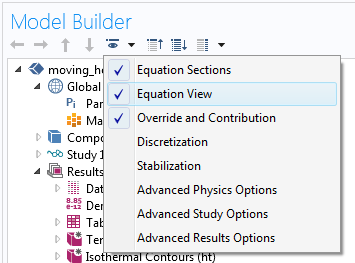
Enabling the Equation View.
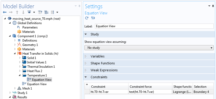
The Equation View for the Temperature node.
The constraint is formulated as ht.T0-ht.Tvar, which implicitly means ht.T0-ht.Tvar = 0. The first term is the prescribed temperature, which you enter as input. The second term is just the temperature degree of freedom cast into a variable. This constrains the temperature to be equal to the given value, unless the given value happens to be the string ht.Tvar. In that case, the symbolic algebra during assembly will reduce the expression to ht.Tvar-ht.Tvar, and further to zero. And with the constraint expression being 0, there is no constraint.
Weak Constraints
In COMSOL Multiphysics, there are actually two possible implementations of a Dirichlet condition. The default case is the pointwise constraint, as referenced above, but you can also use a weak constraint. In the weak constraint, equations are added rather than removed. The heat fluxes needed to enforce the prescribed values of the temperature are then added as extra degrees of freedom (Lagrange multipliers).
You can use essentially the same trick to make a weak constraint conditional, with just a small twist weaved into the mix. Using weak constraints requires that you first enable the Advanced Physics Options.
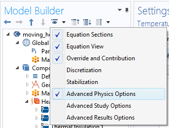
Enabling the Advanced Physics Options.
When weak constraints have been selected in a node within a physics interface, there will be extra degrees of freedom for the Lagrange multiplier. In our case, the degree of freedom has the name T_lm.
If the same expression for the temperature as that shown above is applied, the extra degree of freedom will not get any stiffness matrix contribution on the part of the boundary where the Dirichlet condition is switched off. The stiffness matrix will thus become singular. To avoid this situation, change if(r < R,450[K],ht.Tvar) to if(r < R,450[K],ht.Tvar-T_lm*1e-2). The multiplier used for T_lm differs between varying models and physics fields, and it may require some tuning.
The reason this works, as a textbook might note, is “left as an exercise to the reader”.
Settings for a conditional Dirichlet condition when using weak constraints.
Robin Conditions
The Robin conditions generally contribute to both the stiffness matrix and the right-hand side. The structure of the stiffness matrix is not affected, but values are added to existing positions. The Robin conditions also appear as weak contributions in the Equation View. Turning these conditions into functions of time, space, and other variables is no different than doing so for Neumann conditions.
It is, however, interesting that by selecting appropriate values, you can actually morph Robin conditions into acting as approximative Dirichlet or Neumann conditions. This is especially important for cases where you want to switch between the two boundary condition types during a simulation.
To create a Dirichlet condition, you assign a high value of the “stiffness”, for instance, a spring constant or heat transfer coefficient. In mathematical terms, this is actually a penalty implementation of the Dirichlet condition. The higher the stiffness, the greater the accuracy of the prescribed value for the degree of freedom. But there is a caveat: A very high stiffness will harm the numerical conditioning of the stiffness matrix. For a heat transfer problem, a starting point for choosing a “high” heat transfer coefficient \alpha could be
where \lambda is the thermal conductivity and h is a characteristic element size.
The same idea can be applied to other physics fields by replacing \lambda with the appropriate material property (i.e., Young’s modulus in solid mechanics). The factor 1000 is just a suggestion and can be replaced by 104 or 105.
If you were to use convection to model the moving 450 K spot from the previous example, you could utilize the settings shown below. The built-in variable h for the element size is applied in the expression.
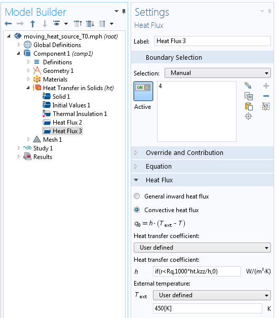
Using a convection condition to prescribe the temperature.
In the good old days, when I first began using finite element analysis, it was sometimes not possible to prescribe nonzero displacements in finite element programs for structural mechanics. The limitation was imposed by the added complexity of the programming. If this was the case, the best option was to use the penalty method by adding a predeformed stiff spring. You wouldn’t want it to be too stiff though; in those days, single precision arithmetic was still in use!
Let’s turn our attention toward approximating a Neumann condition. We want a heat flux that is independent of the surface temperature. In the case of heat transfer, the Robin condition states that the inward heat flux q is
where \alpha is the heat transfer coefficient, T is the temperature at the boundary, and T_{\textrm{ext}} is the external temperature.
So if T_{\textrm{ext}} is much larger than the expected temperature on the surface, then q \approx \alpha T_{\textrm{ext}}. The strategy is then to select an arbitrary, very large T_{\textrm{ext}} and compute a suitable heat transfer coefficient, as highlighted below.
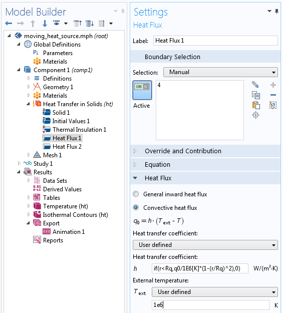
Using a convection condition to prescribe the heat flux.
Designers actually use this principle to introduce a fixed force into real-life mechanical components: a prestressed long weak spring. If the predefomation of the spring is much larger than the displacement of the parts to which the spring is connected, the force in the spring will be almost constant.
Addressing Discretization Errors
When a boundary condition is limited by a Boolean expression like if(r < R,..., then it is more than likely that the border of the region to which it is applied will not follow the edges of the mesh elements. This will introduce discretization errors.
For a Neumann or Robin condition, a numerical integration is performed over each finite element. The value of the function is evaluated at a number of discrete Gauss points in the element. If the size of the mesh elements is large in comparison to the geometrical size of the load, then the exact number of Gauss points covered by the load can significantly affect the total load. As such, there should be several elements on the patch covered by the load at any instant.
A small change in the location of the load may alter the number of contributing integration points. (In reality, the number of integration points is larger.)
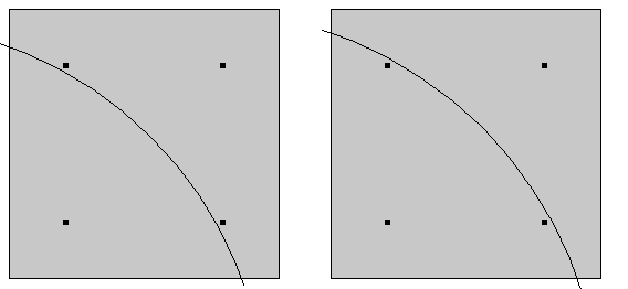
Dirichlet conditions, at least in the pointwise sense, are instead applied to the mesh nodes. In the figure below, the temperature distribution and heat flux are shown for a certain time when simulating the moving circular spot with a prescribed temperature of 450 K. In front of the hot spot, a darker shade with 260 K is visible. Since the initial and ambient temperatures in the simulation are 293 K, this is not expected. It is a numerical artifact that is related to the fact that not all nodes on each element have a Dirichlet condition. At a discontinuity in Dirichlet conditions, there will be singularities. This is a topic of discussion in a previous blog post. Refining the mesh will reduce such an effect.
The green arrows in the following figure represent the nodes at which an influx of heat is created as a reaction to prescribing the temperature. With the mesh density in the model, the approximation of a semicircle will be rather rough.
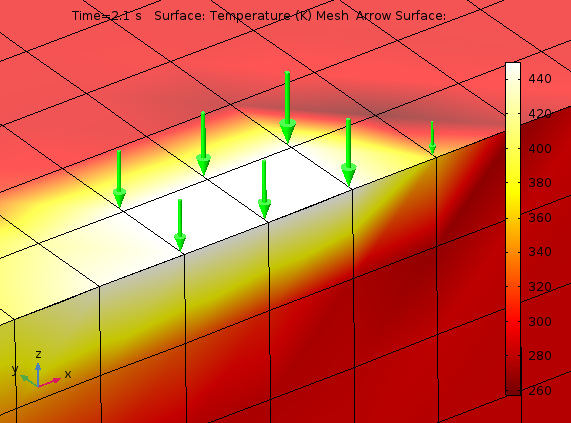
Temperature distribution and heat flux around the semicircular prescribed temperature.
Solution Dependency in Boundary Conditions
There are many ways in which the solution can enter your boundary conditions. This will generally introduce nonlinearities, which are automatically detected by COMSOL Multiphysics.
As an example, let’s look at a beam featuring a support that is placed slightly below it, inhibiting further movement after a certain deflection. This can be implemented with a conditional Dirichlet condition via a Prescribed Displacement/Rotation node in the Beam interface.
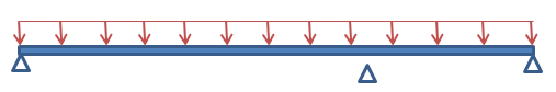
Beam with a deflection, controlling support and distributed load.
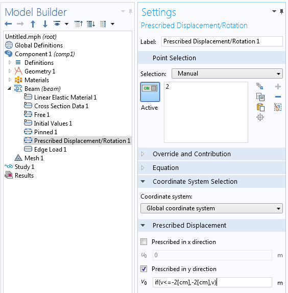
Settings prescribing that the beam should stop at a deflection of 2 cm.
The analysis shows the expected behavior. At lower loads, the deflection shape is symmetric, whereas at higher load levels, the point on the beam where the extra support is located will stop moving. At the final load level, the beam will even undergo a change of sign in the curvature. This is visible in the deformation plot, but it is shown more clearly in a bending moment graph.
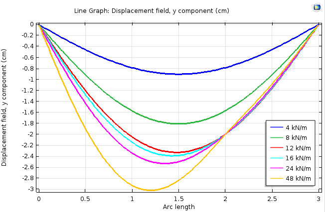
The beam displacement at the support point stops at 2 cm.
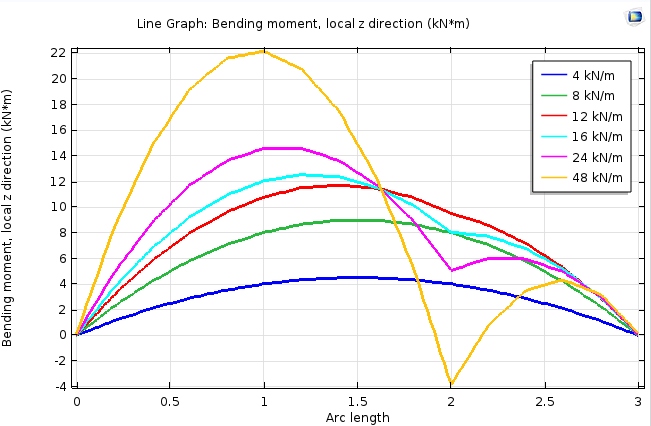
Bending moment along the beam for various load levels.
The approach highlighted here is rather crude and the iterative solution may not have good convergence properties. A more stable implementation is to use a highly nonlinear spring at the support point, so that the reaction force is a continuously differentiable function of the displacement. This is actually similar to how penalty contact is implemented in the Solid Mechanics interface.
Concluding Thoughts on Utilizing Boundary Conditions in COMSOL Multiphysics
COMSOL Multiphysics gives you access to very powerful mechanisms for prescribing nonstandard boundary conditions. Today, we have provided you with a few examples of what you can do with these conditions.
For those who are interested in analyzing a model with a traveling load, take a look at the Traveling Load tutorial model, available in our Application Gallery.
If you have additional questions on how to prescribe nonstandard boundary conditions within your own modeling processes, please contact us today.


Comments (27)
Ivar Kjelberg
July 1, 2016Hi Henrik
Thanks for an excellent BLOG on very useful “Tricks” to handle complex physics cases in COMSOL. I was familiar with some of them, but had not really thought of all other combinations you are showing here 🙂
You have such a powerful tool and there is so many engineers and scientist not even knowing about COMSOL, but too bad for them 🙂
Sincerely
Ivar
Hassan Abdelkariem
July 6, 2016Thank you! it is such useful BLOG.
Eric
November 29, 2016Hi Henrik,
I have a question about solution dependent boundary condition (BC). I am solving a Poisson-continuity fully coupled equation involving two variables, which are electric potential (phi) and space charge density (rho). I am able to obtain converged results when using Dirichlet BC for phi. However, when I change the Dirichlet BC to a variable BC, which depends on the variable rho and gradient of phi, the stationary solver does not lead to convergency. I guess the model is not well posed after using the variable BC.
I have no prior experience in implementing a variable BC, so any suggestion will be greatly appreciated.
Eric
Henrik Sönnerlind
November 29, 2016 COMSOL EmployeeEric,
Please send questions of this type to support, or post them on the user forum. I think it would be necessary to attach a model to get help in either case.
Regards,
Henrik
Mohammadreza Samieegohar
June 2, 2017thank you, it was so useful for me.
Sagar Deshmukh
August 27, 2017In electric current, there is no term like fixed current for Neumann boundary condition
Henrik Sönnerlind
August 28, 2017 COMSOL EmployeeSagar – The name of the Neumann boundary condition in the Electric Currents interface is ‘Normal Current Density’. The table in the beginning of the blog post is more conceptual.
Regards,
Henrik
fedaoui kamel
September 7, 2017thank you, it was so important for me
Junaid Baig
February 11, 2018Thank you for this post. Could you please solve following doubt for me?
How does COMSOL exactly solve for location of heat source with the equation q0*(1-(r/R)^2)?
Henrik Sönnerlind
February 12, 2018 COMSOL EmployeeJunaid,
We do not really have to solve anything here. The expression is evaluated over the whole boundary at each time step. At the time of evaluation of the expression, the coordinates of the location where it is evaluated are compared against (1-(r/R)^2). The variable r is the distance from a certain location, which changes in time.
Depending on the type of contribution that is computed, the point of evaluation can be a mesh node or an integration point (Gauss point).
Regards,
Henrik
DJEMMAL Faouzi
May 21, 2018what are the boundary conditions that I have to use in electrostatic regime when I solve the Poisson’s equation?
Thank you
Henrik Sönnerlind
May 24, 2018 COMSOL EmployeeHi Djemmal,
If you want to discuss boundary conditions in general, please post your questions in the user forum: http://www.comsol.com/forum
Regards,
Henrik
zoubir bekkari
August 29, 2018Thanks for an excellent BLOG on very useful
Matias Andres Arntzen
June 16, 2019Hello, i would like to know how can i do to simulate a continous workload moving through a microwave dryier conveyor. I`ve design the microwave dryier but i dont know how to make the workload move. Thank you very much
Henrik Sönnerlind
June 17, 2019 COMSOL EmployeeHi Matias,
To get help, you can either contact support ( https://www.comsol.com/support ), or post your question in the user forum ( http://www.comsol.com/forum ). In either case, I think you will have to provide some more detail, for example sketches.
This said, there are in principle two possible approaches:
1. You actually move the material, that is the mesh.
2. You incorporate a convective term in your equations, so that a time derivative du/dt is replaced by du/dt + velocity * grad(u)
Regards,
Henrik
Susheel Pandey
November 26, 2019Sir I am trying to solve “Laser Heating of Silicon Wafer” https://www.comsol.co.in/model/laser-heating-of-a-silicon-wafer-13835#comsol54
But Sir while “Solving ” it shows two error (1) Unknown function/operator Name – “Pulse” (2) Feature -Time-Dependent Solver1 (sol1/t1).
Pulse :- may be becoz in value of Fa (in Boundry load ) its showing some error pls .As given in Pdf in your website I have followed every step .
Please Tell me if it is correct ” if(BehindFirstLoad, -LoadIntensity*Pulse(X-LoadSpeed*t),0) ” .
Brianne Christopher
December 2, 2019 COMSOL EmployeeHello Susheel,
Thank you for your comment.
For questions related to your modeling, please contact our Support team.
Online Support Center: https://www.comsol.com/support
Email: support@comsol.com
Jing Yuan
July 11, 2020Hi, Henrik.
Can I ask a question?
In your post, does the Robin Boundary Condition look like: k*dT/dx=a*(T0-T)? I was trying to implement such a boundary condition in Comsol, but the result shows the convective heat flux is much different from the conductive heat flux.
What I did was setting q0=h(Text-T) as convective heat flux, I assume it should be equal to k*dT/dx at the boundary. So I’m not sure if this is the correct way.
Thanks a lot. Stay safe.
Jing
Henrik Sönnerlind
July 13, 2020 COMSOL EmployeeHi,
Even if your equation is 1D, you need to take also the orientation of the normal into account (the signs would be different at the left and right ends of the interval).
Anyway, this condition is built-in in the Heat Transfer in Solids interface. If you are doing your own equation based model, you can compare with what is built-in.
Note that the temperature gradient inside the material (from which I think is what you are computing the ‘conductive heat flux’) will only match h(Text-T) to the extent that the solution can be represented by the shape functions used. A finer mesh should give a closer match.
Ghulam Anwer
August 10, 2022Hii…quite helpful this blog is…can anyone suggest to me an equation to change coordinate in both x & y directions at a time?
Henrik Sönnerlind
August 15, 2022 COMSOL EmployeePlease send your question to support or to the user forum, preferably with a longer description.
John sunil kumar Palle
July 7, 2023Thank you for the information. Iam exactly using a temperature boundary condition that needs to be cut off after a particular time. I have a query on the term ‘Tvar”. where exactly have you defined it? I want to apply the following BC “if((intop1(T2)<473),Tempbc(t)[1/s] else no Boundary condition. Please respond
Henrik Sönnerlind
July 10, 2023 COMSOL EmployeeHi,
If you look in Equation View for a Temperature node in Heat Transfer in Solids, you will see that the constraint is written in terms of a variable called ht.Tvar. The constraint reads
ht.temp1.T0-ht.Tvar
where ht.temp1.T0 is the temperature value you enter.
If you check the definition of ht.Tvar, it will for most cases simply be equal to the temperature DOF ‘T’. The advantage of using a local variable instead is that the expression is insensitive to the actual name of the temperature DOF.
Your expression should be something like if((intop1(T2)<473),Tempbc(t)[1/s],ht.Tvar)
John sunil kumar Palle
July 20, 2023Thanks. It worked. Appreciate your response.
Tarek Nehila
July 14, 2023Good morning sir
can you send me the project
nehila.tarek@univ-bechar.dz
best regards
George Yin
October 14, 2024Hi Henrik
I would like to understand the principle behind setting Dirichlet boundary conditions under weak constraints as described in the blog. My understanding is that the unconstrained regions increase the dimensionality of the Lagrange multiplier vector, enhancing the singularity of the stiffness matrix. It seems that the way to solve this issue is to eliminate these degrees of freedom. Could you please explain why specifying the displacement of the unconstrained regions as ht.Tvar minus 0.01 times the Lagrange multipliers achieves this?
Yin
Mulubrhan Tsegabruk Berhe
January 8, 2025Hello
I am working in a liquid-gas membrane contactor while I try to give a boundary for the flux in the transport of diluted species it does not allow me to add the membrane tube interface where the flux takes place would give me your insight thank you in advance.