

Today we continue our discussion on the weak formulation by looking at how to implement a point source with the weak form. A point source is a useful tool for idealizing the situation where a source is concentrated in a very small region of the modeling domain. We will find that it is very convenient to set up such a point source using the weak form.
The Mathematics of a Point Source
Consider a one-dimensional domain on the x-axis with a source localized around x = 0. We can plot the strength of the source as a function of x and it may look like this:
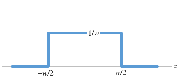
Here, we have assumed that the strength has a constant value of 1/w within the interval [-w/2, w/2] and is zero everywhere else. This gives a rectangular shape of width w and height 1/w, as shown in the figure above. The function is often called a rectangular, top-hat, or sometimes, a disc function. The total strength of the source is given by the area of the rectangle, which is unity.
For linear systems, if we only care about what happens far away from the source where \left| x \right| \gg w, then the actual shape of the source strength does not matter much, as long as the area beneath that shape is the same. Furthermore, we are free to make w progressively smaller and smaller: the width of the rectangle decreases while its height increases in such a way that the total area remains the same, as shown in the graph below.
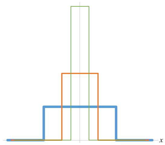
The localized source represented by the blue curve is progressively made thinner and taller (the orange and green curves), while maintaining the integrated strength of unity.
Eventually, we arrive at a rectangle that is infinitesimally thin and infinitely tall, but still has a well defined area of unity. This leads us to the so-called delta function \delta(x) and, correspondingly, the localized source now becomes an idealized point source of unit strength.
The delta function has some convenient properties. Its value is zero everywhere except at the origin:
\infty \mbox{ for } x=0\\
0 \mbox{ elsewhere}
\end{array} \right.
Integrating the product of a delta function and another function just extracts the value of the latter function at the origin:
A point source at a general position x=a can be obtained by a simple coordinate shift of the delta function \delta(x-a). We have
\infty \mbox{ for } x=a\\
0 \mbox{ elsewhere}
\end{array} \right.
and
It is also easy to generalize the delta function and the corresponding point source to higher dimensions. For example, in 2D, we have
\infty \mbox{ for } x=a, y=b\\
0 \mbox{ elsewhere}
\end{array} \right.
and
(1)
Implementing a Point Source Using the Weak Form
This tutorial solves the Poisson equation on a unit disc with a point source at the origin. The equation reads
(2)
where u is the dependent field variable to be solved.
At first sight it may not be obvious how to discretize this equation to be solved numerically. What value do we put at the origin for the source term on the right-hand side? The value of the delta function is infinite there, but computers don’t like infinities!
Here, we will see that the weak formulation comes in handy. Recall that in this introductory blog post on the weak form, we multiply the differential equation to be solved by a test function and integrate over the entire domain (See Eq.(4) in that post). We can follow the same procedure here to solve Eq. (2). After multiplying by a test function \tilde{u}(x,y) and integrating over the unit disc domain, the right-hand side of Eq. (2) simply becomes
(3)
by using the integration property of the delta function given in Eq. (1). This gives us something very easy to implement in COMSOL Multiphysics.
Start with a new 2D model with the Weak Form PDE physics interface and a Stationary study. Draw a unit circle centered at (0,0) and draw a point there as well. Set the Weak Expressions field under the default Weak Form PDE 1 feature to -test(ux)*ux-test(uy)*uy. This takes care of the left-hand side of Eq. (2) in exactly the same fashion as for the 1D case discussed in this previous post.
Now, for the point source on the right-hand side, \tilde{u}(0,0), we simply add a point Weak Contribution node and select the point at the origin. For the Weak expression, we enter test(u). It’s that simple for the point source!
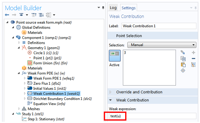
It may be worth noting that by entering test(u), we set the strength of the point source to unity. For any other source magnitude, simply multiply by a factor. For example, the expression 2*test(u) gives a point source of strength 2.
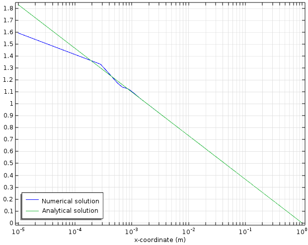
After finishing the set-up with a Dirichlet boundary condition at the perimeter of the circle, we can solve the model and observe the same solution as seen in the point source tutorial mentioned above:
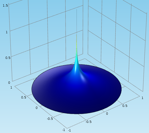
Also as seen in the tutorial, the numerical solution (blue curve) matches the analytical solution (green curve) very well, except near the origin where a singularity occurs:
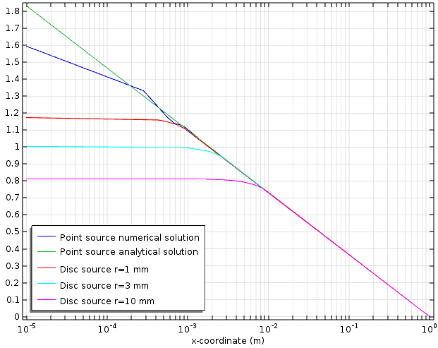
As mentioned earlier, the point source provides a convenient idealization of a localized source in situations where we only care about the solution far away from the source. We illustrate this point with the following graph, where we have added three more curves to the graph above. These three curves are numerical solutions to the same Poisson equation in the same unit disc domain, but with various sizes of top-hat, or disc, shaped sources replacing the point source. The integrated strength of each top-hat source is calibrated to unity by setting its height to one over its area, in the same fashion as in the 1D case shown in the image above. As we see clearly from the figure below, all solutions are indistinguishable from one another far away from the sources. (In this example for x \gg 10 \, mm.)
Conclusion
Here, we have demonstrated the ease of creating point sources using the weak form. The numerical difficulty in the representation of the delta function is circumvented with a simple integration. In upcoming posts we will look at discontinuities and boundary conditions. Stay tuned!


Comments (11)
Vishwas Nesarikar
August 25, 2015Very nice explanation. Thanks
Perry Gao
November 11, 2015Dear Chien,
Thanks for your great post!
I recently met some problem in implementing ‘identity pairs’ to realizing discontinuous boundary conditions in weak form pde.
Is this going to appear in your next blog?
Thanks!
Perry
Carolina Montoya-Pachongo
November 28, 2016Dear Chien, wonderful posts about the weak form of PDEs. I can see you did not publish posts anymore. Is someone else in charge of the following topics: discontinuities and boundary conditions? Many thanks.
Chien Liu
November 28, 2016 COMSOL EmployeeDear Carolina, yes we do hope to continue the blog series in the future. Stay tuned! Chien
Dhiman Das
February 17, 2018Dear Liu, while choosing Weak Contribution, I am not able to select the point in the middle of the circle. Am I doing something wrong? Please help.
Dhiman Das
February 17, 2018Dear Chien, I am not able to select the point in the middle of the circle as the weak contribution. Am I doing something wrong?
Chien Liu
February 17, 2018 COMSOL EmployeeDear Dhiman, Please make sure that you add a “point” Weak Contribution (under the sub-menu “Points”), not a “domain” or “boundary” Weak Contribution. Hope this helps. Sincerely, Chien
Bacha Munir
October 10, 2018Your explanation is very nice. Thank you so much. Please, also explain for 2d boundaries/surfaces. Specially for weak form of naveir stokes equations, which need to solve for three variables, u,v and p. Can you please explain how we can implement weak constraints on air liquid interface (elliptical shape). directly while solving the NS equations. Thanks.
Brianne Costa
October 10, 2018 COMSOL EmployeeHello Munir,
Thanks for your comment.
For questions related to your modeling, please contact our Support team.
Online Support Center: https://www.comsol.com/support
Email: support@comsol.com
Deepa
June 11, 2021Dear Chien,
Thanks a lot for the interesting post. I tried to implement point sinks along the length of a pipe by coupling the
Transport of diluted species physics and weak form PDE.
But I am facing the issues that I have posted here
https://www.comsol.co.in/forum/thread/291241/solution-not-converging-point-sink-implementation.
Could you please have a look?
Brianne Christopher
June 11, 2021 COMSOL EmployeeHi Deepa,
Thank you for your comment! Please email support@comsol.com or go to comsol.com/support for assistance with your modeling problem.
Best regards,
Brianne