In some applications, particularly within the MEMS field, it is important to study the sensitivity of a device’s eigenfrequencies with respect to a variation in temperature. In this blog post, we show how to do this using COMSOL Multiphysics® version 5.3. We also explore effects like stress softening, geometric changes, and the temperature dependence of material properties.
Studying Temperature-Dependent Eigenfrequencies
Some devices require a very high degree of frequency stability with respect to changes in the environment. The most common parameter is temperature, but the same type of phenomena could, for example, be caused by hygroscopic swelling due to changes in humidity. In very high precision applications, the frequency stability requirements might specify a precision at the ppb (parts-per-billion, 10-9) level. Setting up simulations that accurately capture such small effects can be a challenging task, since several phenomena can interact.
Rectangular Beam Example
Consider a rectangular beam with the following data:
| Property | Symbol | Value |
|---|---|---|
| Length | L | 10 mm |
| Width | a | 1 mm |
| Height | b | 0.5 mm |
| Young’s modulus | E | 100 GPa |
| Poisson’s ratio | ν | 0 |
| Mass density | ρ | 1000 kg/m3 |
| Coefficient of thermal expansion, x direction | αx | 1·10-5 1/K |
| Coefficient of thermal expansion, y direction | αy | 2·10-5 1/K |
| Coefficient of thermal expansion, z direction | αz | 3·10-5 1/K |
| Temperature shift | ΔT | 10 K |
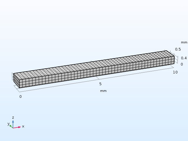
The beam geometry and mesh used in the example.
The material parameters have values that are of the same order of magnitude as those for many other engineering materials. To better separate the various effects, Poisson’s ratio is set to zero, but this assumption does not change the results in any fundamental way. Orthotropic thermal expansion coefficients are used to highlight some properties of the solution.
To analyze the effect of thermal expansion, add a Prestressed Analysis, Eigenfrequency study.
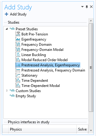
Adding the Prestressed Analysis, Eigenfrequency study.
This study consists of two study steps:
- A Stationary study step that computes the displacements and stresses caused by the thermal expansion
- An Eigenfrequency study step in which the previously computed solution is used
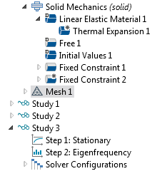
The two study steps shown in the Model Builder tree.
To compute the reference solution, you either add a separate Eigenfrequency study or run the same study sequence, but without thermal expansion.
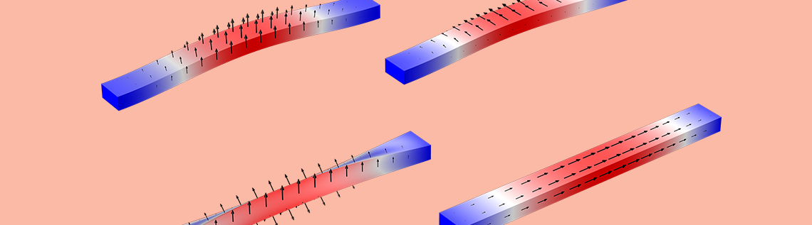
Eigenfrequencies of Doubly Clamped and Cantilever Beams
The eigenfrequencies of the beam have been calculated for two different types of boundary conditions:
- A doubly clamped beam
- A cantilever beam, where one end is fixed and the other end is free
The doubly clamped beam results are shown below.
| Mode Type | Eigenfrequency, Hz | Eigenfrequency, Hz ΔT = 10 K |
Ratio |
|---|---|---|---|
| First bending, z direction | 50713.9 | 50425.1 | 0.9943 |
| First bending, y direction | 97659.6 | 97526.2 | 0.9986 |
| First twisting | 266902 | 266917 | 1.00006 |
| First axial | 500000 | 500025 | 1.00005 |
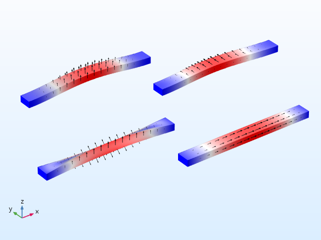
Mode shapes for the doubly clamped beam.
The following table shows the cantilever beam results.
| Mode Type | Eigenfrequency, Hz | Eigenfrequency, Hz ΔT = 10 K |
Ratio |
|---|---|---|---|
| First bending, z direction | 8063.79 | 8066.92 | 1.00039 |
| First bending, y direction | 16049.1 | 16053.7 | 1.00028 |
| First twisting | 132233 | 132265 | 1.00025 |
| First axial | 250000 | 250050 | 1.0002 |
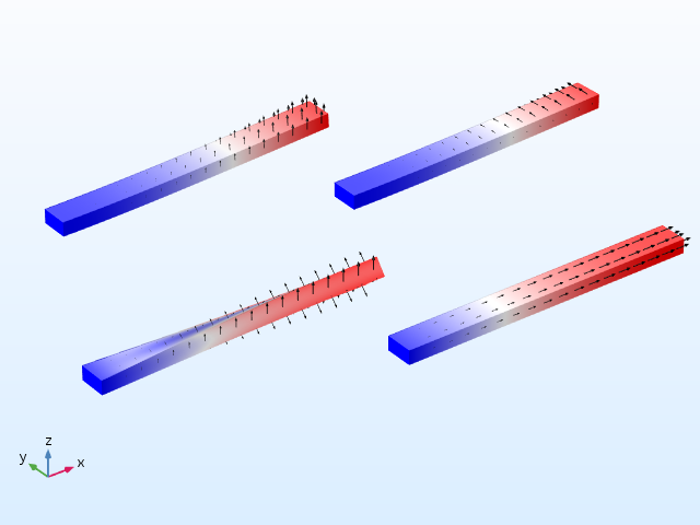
Mode shapes for the cantilever beam.
The first thing to note is that the bending eigenmodes for the doubly clamped beam stand out and have a strong temperature dependence. The change is 0.6% in the first mode. For all other modes, the relative shift in frequency is significantly smaller. If you make the beam thinner, this difference would be even more pronounced. The reason for this behavior is discussed in the following sections.
Examining the Stress-Softening Effect
In the case of the doubly clamped beam, the thermal expansion causes a compressive axial stress. With the given data, the stress is -10 MPa (computed as EαxΔT). This stress causes a significant reduction in the stiffness of the beam — an effect often called stress stiffening, since it typically occurs in structures with tensile stresses. However, compressive stresses soften the structure.
Another way of looking at this is by performing a linear buckling analysis. You can do so by adding a Linear Buckling study to the model and using the thermal expansion caused by ΔT = 10 K as a unit load. You will then find that the critical load factor is 80.
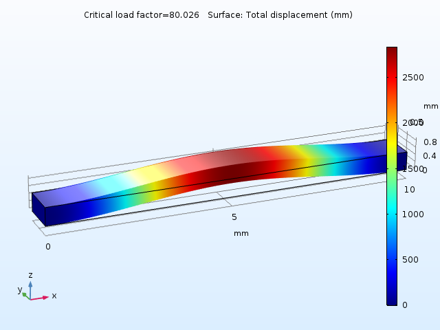
The first buckling mode.
With a linear assumption, the beam becomes unstable at an 800 K temperature increase. At the buckling load, the stiffness has reached 0. Assuming that the stiffness decreases linearly with the compressive stress, the stiffness at ΔT = 10 K should be reduced by a factor of
Since a natural frequency is proportional to the square root of the stiffness, you can estimate the decrease to \sqrt{0.9875}=0.9937, which matches the computed value of 0.9943 well.
Stress softening also affects the twisting and axial modes, but the effect is not as obvious as it is in the bending modes.
Evaluating How a Geometry Change Affects the Frequency
In the cantilever beam, no stresses develop when it is heated, as it simply expands. In this case, the frequency shift is due solely to the change in geometry — an effect that is much smaller than the stress-softening effect.
The natural frequencies for the bending, torsional, and axial vibration of a beam have the following dependencies on the physical properties:
Here, the following variables have been introduced:
- I = Area moment of inertia around the bending axis
- G = Shear modulus
- K = Torsional modulus
- J = Polar moment of inertia around the beam axis
It is assumed that the initial dimensions of the beam are L0 x a0 x b0, where a0 > b0. After thermal expansion, the size is L x a x b.
The expansions (strains) in the three orthogonal directions are called εx, εy, and εz; respectively. In this case, they are linearly related to the thermal expansion by εx = αxΔT, εy = αyΔT, and εz = αzΔT; but in principle, it could be any type of inelastic strain.
The geometric properties scale as:
A& = ab = a_0b_0(1+\epsilon_y)(1+\epsilon_z)\\
I_y& = \frac{ab^3}{12} = \frac{a_0b_0^3}{12}(1+\epsilon_y)(1+\epsilon_z)^3\\
I_z& = \frac{ba^3}{12} = \frac{b_0a_0^3}{12}(1+\epsilon_z)(1+\epsilon_y)^3\\
K& = \frac{ab^3}{3}F_1(a/b) \approx \frac{a_0b_0^3}{3}F_1(a_0/b_0)(1+\epsilon_y)(1+\epsilon_z)^3\\
J& =\frac{ab^3+ba^3}{12}=\frac{a_0b_0^3(1+\epsilon_y)(1+\epsilon_z)^3+b_0a_0^3(1+\epsilon_z)(1+\epsilon_y)^3}{12} \end{align}
The mass density also changes. Since the same mass is now confined in a larger volume,
By introducing these expressions into the formulas for the natural frequencies, you arrive at the following expected eigenfrequency shifts:
Since the thermal expansions are very small, the approximate first-order series expansions can be expected to be accurate.
For the torsional vibrations, the situation is slightly more complicated, since the powers of a and b are mixed in the expression for the polar moment J. But if you make use of the fact that a = 2b for this geometry, then it is possible to derive a similar expression.
Now, compare the computed frequency shifts with the analytical predictions for the cantilever beam. The results are shown in the table below and the agreement is very good.
| Mode Type | Computed | Predicted |
|---|---|---|
| First bending, z direction | 1.00039 | 1.00040 |
| First bending, y direction | 1.00028 | 1.00030 |
| First twisting | 1.00025 | 1.00025 |
| First axial | 1.00020 | 1.00020 |
Analyzing the Effects of Constraint Modeling
The fixed constraints at the ends of the beam cause local stress concentrations when the temperature is increased, as the transverse displacement is constrained.
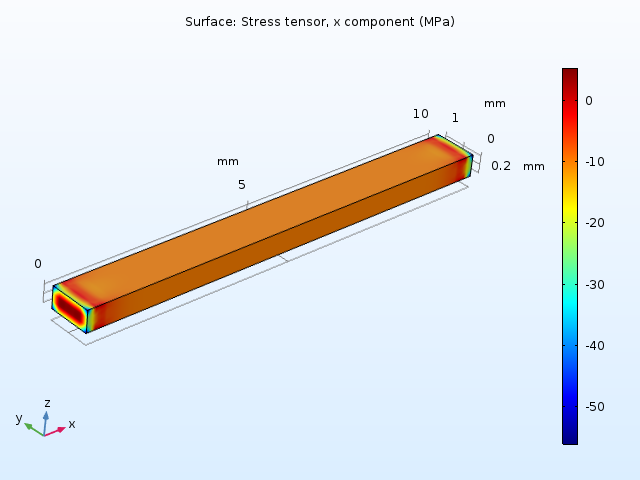
The axial stress in the doubly clamped beam caused by a 10 K temperature increase.
This can have two effects:
- Stress stiffening might be induced in a component that is expected to experience only volumetric changes
- The cross section dimension is no longer constant, due to the restrained transverse displacement (as in the example above)
To determine what effects the constraints should have, you must rely on your engineering judgment. Usually, the component and its surroundings are subject to temperature changes. In this situation, the possibility to add a thermal expansion to constraints in COMSOL Multiphysics comes in handy. Let’s see how the solution is affected.
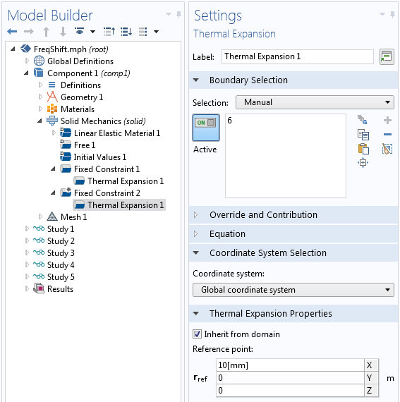
Thermal expansion added to the fixed constraints for the doubly clamped beam.
For the cantilever beam, the results now change so that they perfectly match the analytical values.
| Mode Type | Fixed Constraints | Stress-Free Constraints | Predicted |
|---|---|---|---|
| First bending, z direction | 1.00039 | 1.00040 | 1.00040 |
| First bending, y direction | 1.00028 | 1.00030 | 1.00030 |
| First twisting | 1.00025 | 1.00026 | 1.00025 |
| First axial | 1.00020 | 1.00020 | 1.00020 |
Including Temperature Dependence in Material Data
In the analysis above, it is assumed that the material data does not depend on temperature. When looking at constrained structures (dominated by the stress-softening effect), this might be an acceptable approximation. However, with the small frequency shifts caused by geometric changes, the temperature dependence of the material must also be taken into account.
In this guide, you can see the temperature dependence of Young’s modulus for a number of metals. The stiffness decreases with temperature. For many materials, the relative change in stiffness is of an order of 10-4 K-1. This means that for a temperature change of 10 K, you can expect a relative change in material stiffness that is of the order of 0.1%. This effect might actually be larger than the geometric effect computed above.
A small note of warning: When measuring the temperature dependence of Young’s modulus, it is important to know whether or not the geometric change caused by thermal expansion has been taken into account. In other words, you must know whether the Young’s modulus is measured with respect to the original dimensions or the heated dimensions.
When it comes to mass density, the situation is easier. When performing structural mechanics analyses in COMSOL Multiphysics, the equations are formed in the material frame. Thus, the mass density should never be given an explicit temperature dependence, since that violates mass conservation.
The coefficient of thermal expansion (CTE) usually increases with temperature. The relative sensitivity is often of the order of 10-3 K-1. This sounds large, but it isn’t usually important when looking at the way the CTE enters the equations.
Most materials in the Material Library in COMSOL Multiphysics come with temperature-dependent material properties. In this example, you manually add a linear temperature dependence to the Young’s modulus with the following steps:
- In the settings for the Basic property group, select Temperature under Model Inputs
- Click Add to see that the variable name to be used is T
- Write an expression for Young’s modulus that is a function of T
Alternatively, you can create a function and call it, with T as the argument.

Adding a linear temperature dependence to the material.
In the settings for the Linear Elastic Material, the Model Input section is now active. You then provide a temperature to be used by the material.
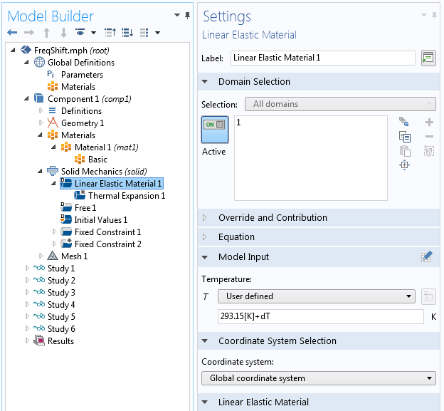
Adding the temperature to the material using Model Input.
After including a reduction of Young’s modulus by 1·10-4 K-1, the resulting frequency shift turns out to be negative, rather than the positive shift observed with a constant Young’s modulus (shown in the table below).
| Mode Type | Stress-Free Constraints Constant E |
Stress-Free Constraints Temperature-Dependent E |
Difference |
|---|---|---|---|
| First bending, z direction | 1.00040 | 0.99990 | -0.00050 |
| First bending, y direction | 1.00030 | 0.99980 | -0.00050 |
| First twisting | 1.00026 | 0.99976 | -0.00050 |
| First axial | 1.00020 | 0.99970 | -0.00050 |
The shift is exactly as expected for all modes — Young’s modulus is reduced by a factor 1·10-3 and the natural frequencies are proportional to its square root. Actually, you can include the change in Young’s modulus in the linearized expressions for the frequency shifts as:
Here, it is assumed that E=E_0(1+\beta \Delta T). The value of the coefficient β is usually negative; In this case, β = -10-4 K-1.
For the common case of isotropic thermal expansion, these expressions simplify to:
A Note on Numerical Accuracy
We are looking for frequency changes that are at the ppm (parts-per-million) level. This means that it is important to avoid spurious rounding errors. There are some actions that you can take to ensure optimal accuracy.
In the settings for the Eigenfrequency node, set Search for eigenfrequencies around to a value of the correct order of magnitude.
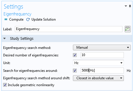
The updated settings in the Eigenfrequency node.
Then, decrease the Relative tolerance in the settings for the Eigenvalue Solver node.
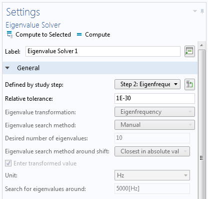
The decreased Relative tolerance in the settings for the Eigenvalue Solver node.
Change only the parameters necessary for capturing the physics. For example, use the same mesh for all studies.
If you have reason to believe that the problem is ill-conditioned, as can be the case for a slender structure, select Iterative refinement in the settings for the Direct solver.
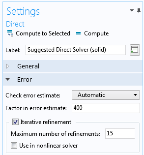
The settings for the Direct solver, showing the option for Iterative refinement.
A Theoretical Excursion into Handling Inelastic Strains Under Geometric Nonlinearity
In version 5.3 of COMSOL Multiphysics®, the method for how inelastic strains are handled under geometric nonlinearity has been changed. A multiplicative decomposition of deformation gradients is the current default, rather than the subtraction of strains that was used in previous versions. This is one key concept to understand why it is now possible to perform this type of analysis with a very high accuracy. Let’s look at a (somewhat artificial) case where the temperature increase is 3·104 K and there are no temperature dependencies in the material properties. This means that the stretches are
resulting in the volume changing by a factor of 3.952.
You can then compare the results from the prestressed eigenfrequency analysis with a standard eigenfrequency analysis on a bigger beam with L = 13 mm; a = 1.6 mm; b = 0.95 mm; and lower density, scaled by a volume factor of 3.952, ρ = 253.036 kg/m3. This of course leads to large increases in the natural frequencies, as the heated object is much larger but with a lower density. The relative changes in frequency for the two approaches are shown in the following table.
| Mode Type | Thermal Expansion and Prestressed Eigenfrequency |
Larger Geometry and Lower Density |
|---|---|---|
| First bending, z direction | 2.2309 | 2.2308 |
| First bending, y direction | 1.8759 | 1.8759 |
| First twisting | 1.6702 | 1.6695 |
| First axial | 1.5292 | 1.5292 |
As can be seen above, the correspondence is in excellent agreement. There is a slight difference in the twisting mode, but that disappears with a refined mesh. Actually, refining the mesh shows that the best prediction is from the prestressed eigenfrequency analysis.
Concluding Thoughts on Studying Eigenfrequencies That Change with Temperature
We have discussed how to accurately determine changes in eigenfrequencies caused by temperature changes with COMSOL Multiphysics, as well as the effects of stress softening, geometric changes, and the temperature dependence of material properties.
Additional Resources
- Check out these blog posts on structural mechanics analysis:
- See updates to the Structural Mechanics Module on the Release Highlights page


Comments (34)
Ivar KJELBERG
May 28, 2017Hei Henrik
Thanks for a very interesting blog. Specially you are “stressing” the delicate settings of the “Reference Temperature” and “Model Temperature” for the materials, and the too often “double effect” arriving when we add T dependence on material and do not check how it applies, in which frame we are.
I’m also noting the new approach to non linear geometry calculations, that might give us some surprises when comparing previous and new models after 5.3. We have many cases when we are comparing ppm level frequency changes due to second order T and sigma effects, for the watch industry. A mechanical “Chronomètre whatch” should have a precision of the order of a few ppm per day! This is high precision mechanics and material science.
We have noticed that if we cannot rely on the precision of the absolute frequency calculated due to mechanical tolerances of the parts we measure, but we have rather good agreements with the relative changes due to Temperature and Stress stiffening/softening that is happening some 100 thousand times, or more, per day in a mechanical watch.
Sincerely
Ivar
Chaitanya Nimmagadda
March 14, 2018Hello Henrik
Thank you for the interesting blog. I am convinced with the shift in eigenfrequency with various conditions. Although, I am not sure on how COMSOL does the analysis.
In study 7 (in the application file) of the model discussed above, when I plot the store solution and the eigenmode, both of them do not have the same dimensions. Ideally, I expected the eigenmode to be displayed on the thermally expanded structure. So in the prestressed eigenfrequency analysis, does the eigenfrequency analysis use the deformed structure with thermal stresses as the initial condition? or does it use any other condition? Any help is much appreciated.
Thanks
Chaitanya
Henrik Sönnerlind
March 15, 2018 COMSOL EmployeeHi Chaitanya,
The problem is formulated on the initial geometry (‘material frame’ in our terminology). This can be seen as a transformation from the thermally expanded state. This approach has the drawback that mode shape, as a default, is plotted on the undeformed geometry.
You can create a mode plot with respect to the deformed geometry by manually superimposing the predeformation in the ‘Deformation’ node.
1. Use an expression for the deformation like
withsol(‘sol2’,u)+multiplier*u.
Here ‘sol2’ is assumed to be the solution containing the preload case. The ‘withsol’ operator can be used to pick up any solution explicitly, and thus allows a blending of results from for example different study steps.
2. Set the ‘Scale factor’ to 1 since you want true scale for the preload deformation.
3. The constant ‘multiplier’ will probably need to be adjusted for each mode in order to get a good visualization. The mode amplitudes can be made more uniform by setting ‘Scaling of eigenvectors’ to ‘Max’ in the ‘Eigenvalue’ Solver node.
Regards,
Henrik
ravi singh
November 6, 2019Dear Henrik,
In the same problem i am interested to obtain the pair of eigenvalue and eigenvectors. Can you suggest the option to get the eigenvalue and corresponding eigenvector.
Thanks in advance.
Ravi
Chaitanya Nimmagadda
March 15, 2018Thank you Henrik for your response.
Following up on my question, in study 2 (in the application file) I enabled and disabled the thermal expansion and I obtained the same set of eigenfrequencies, which is what I expected.
Similarly, in study 7, I set “beta” to be zero, ensuring modulus to be constant, in order to look at the frequency shift just due to thermal expansion. I disabled thermal expansion in both the study steps under the modify physics tree and I obtained the same set of frequencies as obtained in study 2. When I included thermal expansion in just the eigenfrequency step and not the stationary step, I expected the frequencies to be same as that from study 2. But, to my surprise, the frequencies are way off from what I expected.
Extending the above analysis, I enabled thermal expansion in the stationary step and disabled in the eigenfrequency step expecting the same results with the case where thermal expansion is enabled in both the steps. But it is not the case.
I am curious to know how modifying the physics tree effects the solutions. Looking forward to your response.
Thanks,
Chaitanya
Henrik Sönnerlind
March 19, 2018 COMSOL EmployeeHi Chaitanya,
If you think about how the equations as set up based on the weak form, the stiffness matrix is generated from the multiplication stress:test(strain). The stress is computed as C:elastic_strain where C is the elasticity tensor.
Without having a thermal expansion in the eigenfrequency step which matches the one used to compute the displacements of the preload step, the elastic strain (and thus the stress) at the linearization point will be way off. This causes a difference in the stiffness matrix and thus in the computed natural frequencies.
Regards,
Henrik
Chaitanya Nimmagadda
March 26, 2018Hello Henrik,
Thank you for your response. To thoroughly understand what was going on, I wanted to take a look at the stiffness matrices, K, for Cantilever without thermal expansion, Study 2 (sol2) and Cantilever with thermal stresses, Study 6 (sol9) using MATLAB live-link. The modulus is same for both the studies. And I obtained the exact same matrices. I expected a difference in the stiffness values as thermal expansion leads to change in the dimensions of the structure. Any insights into what is going on is much appreciated.
Thanks,
Chaitanya
Chaitanya Nimmagadda
March 27, 2018Hello Henrik,
I also compared sol2 with sol15 (dT=30000K) and saw a maximum change in the order of 2.9802e-8
Best,
Chaitanya
Henrik Sönnerlind
March 27, 2018 COMSOL EmployeeHi Chaitanya,
I see significant differences (relative changes of the order 1e-4) when I check the stiffness matrices in the GUI (using an Assembly node and Derived Values->System Matrix) for sol2 and sol9. It seems like you have made a mistake in the export. My best guess is that you got the matrix without geometric nonlinearity or wrong linearization point.
Regards,
Henrik
Chaitanya Nimmagadda
March 29, 2018Hello Henrik,
If I understand it correctly, we are trying to find the eigenvalues of the equation Mx”+Kx=0. With temperature change the structure deforms thereby changing the K matrix to say K’. Now we solve the new equation to Mx”+K’x=0 to find the new set of eigenvalues. The new equation will account for deformation and the thermal stresses also taken into account into K’ while forming the stiffness matrix. Will there be any remeshing done between steps to account for change in shape?
Thanks,
Chaitanya
Chaitanya Nimmagadda
April 3, 2018Hello Henrik,
Can you tell me the equation COMSOL solves for in the second step (eigenfrequency) ? I want to understand how the geometric and pre-stress affects the system matrices (M & K).
Thank you for your time.
Chaitanya
Henrik Sönnerlind
April 3, 2018 COMSOL EmployeeHello Chaitanya,
The equations are always formulated in the undeformed configuration. Thus, the mass matrix is not affected. The stiffness matrix is changed because of the effects of initial stress and strain.
To actually compute the effects on the stiffness matrix requires an element-by-element evaluation, as is done in the assembly phase. Not all elements of the matrix scale in the same way.
To derive the formulation, you would have to set up the virtual work expressions in the the deformed configuration, and then change variables in the integrals in order to transform them to the original configuration.
Regards,
Henrik
Chaitanya Nimmagadda
June 20, 2018Hello Henrik,
Thank you again for the interesting blog and your responses. In addition to what you have shown in your blog, I also looked at prestressed frequency domain analysis (longitudinal excitation) of the cantilever beam and the peak in transmission response is consistent with the predicted results and prestressed eigenfrequency analysis.
Thanks,
Chaitanya
Bartłomiej Chojnacki
April 29, 2020Hello,
is it still possible to get this model .mph for 5.3 COMSOl version? I think it was deleted from model library, only presentation left…
Regards,
Bartlomiej
Henrik Sönnerlind
April 29, 2020 COMSOL EmployeeHi Bartlomiej,
In Application Galleries, it is only possible to find model files for the last three versions, which today means 5.3a, 5.4, and 5.5.
(Actually, those files were not visible either, but that is fixed now.)
Regards,
Henrik
Dave Van Tol
July 20, 2020Henrik, thank you for this example. I would like to extend this analysis a bit, I’m hoping you might have a tip or two.
I’d like to set a heat flux boundary condition on a surface, then run a transient analysis to a specific time stamps. Then I’d like to run an eigenfrequency analysis at each of the specified time stamps.
I think this requires me to perform a Study, then use the results of that Study as the starting point for another study. I don’t know how to do that. Any tips?
Thanks in advance!
Henrik Sönnerlind
July 21, 2020 COMSOL EmployeeHi Dave,
In principle, you do the following:
1. Run the thermal transient in a separate time-dependent study. Here, you only solve for the temperatures.
2. Create a new study of Eigenfrequency type (with geometric nonlinearity selected to capture the thermal expansion effects). Here, you only solve for Solid Mechanics.
3. In this second study, go to the section ‘Values of Dependent Variables’ and make sure that you point to the heat transfer study.
4. Add ‘t’ as a parameter under ‘Parameters’.
5. Add a ‘Parametric Sweep’ to the second study. Select ‘t’ as the parameter, and enter the list of time stamps at which you want to perform the eigenvalue analysis. ‘t’ is recognized as the time in the referenced study, so the correct temperatures will be retrieved.
If you need more advice about this, I suggest that you move to the user forum, or go through support.
Regards,
Henrik
Dave Van Tol
July 21, 2020Thank you Henrik! I’ll give it a try.
Dave Van Tol
December 9, 2021I made this work back in 2020, and promptly lost my hard drive before I backed it up. I didn’t figure it out right away, and that’s an understatement. So when I needed to recreate this in 2021, I approached with trepidation. And rightly so, because it took me many attempts to get this to work.
For future reference (for myself and anyone else that wants to do this), here is the sticking point. In Henrik’s step 3, I had to select “Interpolated” for the field “Time(s).” And in the field that appears when I select “Interpolated,” I enter the variable “t.” COMSOL flags that variable t as a cyclic dependency. It also marks the Eigenfrequency analysis with a red X to flag the error, but it does the calculation anyway.
Stefano Mariani
January 7, 2024Dear Dave, thank you for your updated comment on your solution to this issue back in December 2021. I am also struggling with this task. In my case, everything seems to work fine as I don’t get any error (I am using COMSOL 5.6), and I get eigenfrequencies solutions. Problem is the computed eigenfrequencies are all identical across any selected value for the parameter “t”, although I am injecting a significant heat-flux in the transient analysis and this causes very relevant displacements to my structure (elongation of a couple of meters for my simple 5-meter-long beam-like object used for testing this procedure). Note that I have pointed the second study (eigenfrequency) to the first study (transient heat transfer), as in point (3) of Henrik above, and I have selected geometric nonlinearity to capture the thermal expansion effects, as in point (2) of Henrik above. I am wondering whether you or Henrik can share any additional tip on this matter? Thank you very much!
EDIT: after a couple days of struggle I finally understood what I was doing wrong. Under “Values of Dependent Variables” I had only pointed to the first study the section entitled “Initial values of variables solved for”. After I also pointed the section “Values of variables not solved for” it is now working, thank you again Dave and Henrik for your helpful comments up here!
Tobias Adam
July 14, 2023Hello dear comsol team, and thank your very much for your work Henrik!
Unfortunately I can’t find any model files in the Apllication galery for this example.
Only a PowerPoint presentation appears in my case.
I use Comsol 6.1.
Thank you very much for your help
Tobias
Henrik Sönnerlind
July 17, 2023 COMSOL EmployeeHi Tobias,
The reason that you could not see any model files is that files that are ‘too old’ are no longer visible. In this case, the blog post was written using version 5.3. I have uploaded a version 6.1 file now, which you should be able to download. Note that this is just an ‘open and save again’ version, so from a modeling point of view, it is the same model as originally used. It does not make use of more recent functionality.
Actually, we are getting many requests for this example. From version 6.2 (later this year), this will be an example in Application Libraries, and as such actively maintained.
Regards,
Henrik
Federico Sordo
December 8, 2023Hello,
thank you for this great tutorial! I am currently working in modal analysis in MEMS devices, and in particular I am studying temperature stability of resonance frequency. Hence I am using the prestressed eigenfrequency study node.
For what concerns the effects of temperature on frequency, apart from temperature dependence of material properties, it is not clear to me how they are implemented. In this sense: how the results of the stationary analysis are used? To assemble the new mass and stiffness matrices for the second step? Does COMSOL compute the “new” density after thermal expansion, with the solution for axial strains, and use this new density to assemble the mass matrix for the second step?
Because I am trying to simulate this effect but in a 2D model, and I cannot get the desired results; I suspect that since the model is 2D (Plane strain with out of plane mode extension), I cannot take into account the change in density due to thermal expansion.
Henrik Sönnerlind
December 12, 2023 COMSOL EmployeeCOMSOL uses a pure ‘Total Lagrangian’ formulation. This means that everything is computed with respect to the original configuration. Thus, the mass matrix does not change. All effects of the static load case enter the stiffness matrix. There are two types of possible nonlinear contributions: One comes from the stresses in the stationary case (“stress stiffening”), and one is a pure geometrical transformation based on the deformation gradient from the stationary case. You can examine the details using Equation View. However, there are quite a large number of operations and transformations along the road.
When you are working in 2D, you can consider using an anisotropic coefficient of thermal expansion with a zero out-of-plane value. Depending on the situation you are modeling, that it can be a correct idealization which avoids strains/stresses to occur in that direction.
Federico Sordo
December 12, 2023Thank you very much for your answer. It is still not perfectly clear how the change in mass density cited in the article can be taken into account. If the thermal expansion is not constrained at all, stress stiffening won’t affect the stiffness matrix; hence all the effects must be taken into account through the geometrical transformation of the stiffness matrix. But how that change in mass density can be considered?
Henrik Sönnerlind
December 12, 2023 COMSOL EmployeeI agree that this is counterintuitive.
An overly simplified way of expressing it is that the volume scale factor can be placed either on the mass matrix or (as inverse) on the stiffness matrix. From an eigenfrequency perspective it does not matter.
If you were to compute a mass matrix based on the new density, then you must also integrate over the deformed volume. If not, there would not be mass conservation. It can actually be shown that the mass matrix in a spatial representation, and the mass matrix in a material representation, are the same. Either you have
integral_over_original_volume(original_density x shape_function x shape_function x dV)
or
integral_over_current_volume(current_density x shape_function x shape_function x dv)
Since the density scales as the inverse of the volume, the result will be the same. And since the mass matrix is not affected by thermal strain (or any other deformation), any changes must appear on the stiffness side.
Federico Sordo
December 12, 2023That is very clear, thank you very much.
If I understood correctly then, the following example should give the idea. Let’s consider a simple case, a constant cross section, free-free bar that is subjected to axial vibrations.
The increase in temperature generates a normalized increase in length by a factor of (epsilon_xx); this should generate a decrease of the overall stiffness of the same factor. This should also generate a decrease in density that cause an increase in frequency (normalized) by a factor (0.5*(epsilon_xx + epsilon_yy + epsilon_zz)). Hence, the geometrical transformations performed on the stiffness matrix should scale the stiffness matrix terms by these factors and eventually produce an overall scaling of (1 +0.5*(-epsilon_xx + epsilon_yy + epsilon_zz)). I also guess that these geometric transformation “scale” the stiffness matrix not isotropically. Could it be something like that?
I am asking this because I am trying to see if I can still perform this kind of prestressed analysis in 2D, by taking into account the effect of the 3 components of the thermal strains; I am trying to understand if the same kind of geometrical transformations are performed in the same way also in 2D.
I think I have 2 options. The first one should be to set the out-of-plane components of the thermal expansion to 0 (to avoid stresses in the out of plane direction) and then just scale the material density of a factor (1-alpha_Z*delta_T), to take into account the out of plane deformation that affect density. The second option would be to compute the eigenfrequency analysis without the prestress, but by manually adjusting both the length of a factor (1+alpha*deltaT) and the density by a factor(1-3*alpha*deltaT). Could any of these work?
Thank you very much in advance, I really appreciate your help.
Henrik Sönnerlind
December 13, 2023 COMSOL EmployeeYou can always use the ‘manual’ approach, like I did in the blog above when comparing results for the super large expansion. That is easy if you have a uniform thermal expansion without, for example, constraint effects. But the built-in should work fine too, as long as you have sorted out what is the physically correct 2D approximation.
Federico Sordo
December 19, 2023Thank you very much. I would like to ask one last thing if possible; how the stress stiffening is implemented? Because from the results I am getting stress also influence shear modes resonant frequency, and I cannot find literature references about this phenomenon.
Henrik Sönnerlind
December 20, 2023 COMSOL EmployeeThe stress stiffening contribution to the stiffness matrix comes from a virtual work expression where the initial stress tensor is multiplied with the variation of the Green-Lagrange strain. So if you would have only an initial stress in the x direction sXX, then
dW = sXX * d(eXX) = sXX * d(u,X + 0.5*(u,X^2+v,X^2+w,X^2)).
Pure shear modes are not often seen. What is usually termed ‘shear modes’ are usually combined with more or less bending. A prestress will then, to some extent, affect also such modes.
Federico Sordo
January 18, 2024Hello,
thank you for your answer, always very detailed and clear.
I was trying to better understand the meaning of the geometric nonlinearity introduced with the prestressed analysis. I read this other article of yours: https://www.comsol.com/blogs/what-is-geometric-nonlinearity/ .
Maybe this comment should be posted under the other article. If so, I apologize in advance.
It looks to me that in the default settings for this kind of study, as well as in the tutorial posted here, the option “Include geometric nonlinearity” is enabled for the Eigenfrequency study only. If I understood correctly, this allow to properly set up the stiffness matrix for the Eigenfrequency analysis, by using the Green-Lagrange strains to perform the geometrical transformation (and stress stiffening contribution). This means that geometrical nonlinear terms are considered in this step.
However, I do not understand the implications of considering this nonlinearities in the eigenfrequency analysis only; if those are relevant for the eigenfequency analysis, how can they be properly taken into account if the initial displacement field is computed with a linear analysis? In which cases this assumption is legit?
Thank you in advance,
Federico Sordo
Henrik Sönnerlind
January 23, 2024 COMSOL EmployeeThe nonlinear terms are important for a correct linearization of the stiffness matrix. But usually the nonlinear terms in themselves (that is, the quadratic contribution to the strain tensor) are small. If the deformations are so large that a geometrically nonlinear analysis is necessary to get a correct result in the prestress loadcase itself, then that step must also be geometrically nonlinear.
Think, for example, about stress stiffening. A strain of 0.001 gives a negligible contribution to the strain tensor, so the prestress solution is virtually linear. However, the contribution to the tangent stiffness matrix at that point from a stress which for a metal is of the order of the yield stress is still large. The stress stiffening term, coming from a geometric nonlinear effect must be used for the eigenvalue problem.
Federico Sordo
January 25, 2024Thank you very much; as always very clear. After many tests though, it looks to me there are some situations in which the strains are still not large enough to justify a nonlinear static analysis, but large enough to still generate some “artificial” effects on the resonant frequency.
Let’s consider this example: a cantilever beam subjected to differential thermal expansion, that causes the beam to bend. Since one end of the beam is free, even if the deflection is high (let’s consider a deflection equal to twice the thickness of the beam), the solutions obtained through linear and nonlinear analyses are practically the same; the engineering strain computed through the linear analysis and the Green-Lagrange strain computed trough the nonlinear analysis are almost identical, showing that in this case, since the end is free, nonlinear effect can be neglected in the static analysis.
However, if then I compute the Green-Lagrange strain for the static analysis, I get a very different result; from my comprehension, I would say that this is normal because in a linear analysis the spatial and material frames coincide; as a consequence, the large rotations at the end of the beam will artificially make those second order terms significant. Consequently, if I then include geometric nonlinearity in the eigenfrequency step, those “artificial” second order effect will affect the stiffness matrix and hence the eigenfrequency.
Am I missing something? Is there a way to avoid this kind of inconsistency without the need to perform a nonlinear static analysis (like a step to recompute the strain in between)? Or the only way to avoid this is to not include geometric nonlinearities in the eigenfrequency step, hence loosing accuracy on any possible stress stiffening effect?
Thank you in advance, have a nice day.
Henrik Sönnerlind
January 30, 2024 COMSOL EmployeeThe safe way is to always include geometric nonlinearity also in the prestress case. For an almost linear case, this will, however, double the solution time, since one extra solution is needed just to ascertain that no correction to the first solution is needed.
The case with the cantilever beam that you mention is particularly nasty. In a linear solution, the displacements are only vertical. That solution will, if uncorrected, give a very large axial tensile force when including second order terms. The center line is extended in an unphysical way.
However, when displacements in a beam exceed approximately half the thickness, the problem should always be considered as geometrically nonlinear. Not taking that into account will be a mistake for any type of analysis.