
If you’re new to uncertainty quantification (UQ), this blog post introduces the concept through a simple resistor example. We go over four of the study types in the Uncertainty Quantification Module, including screening, sensitivity, propagation, and reliability, in the context of designing a resistor.
What is Uncertainty, and Why Should Engineers Care?
Consider Roberto Baggio, the elite soccer player who missed a decisive penalty kick in the 1994 FIFA World Cup® final. The reason for that dramatic miss may lie in the hidden variables: the randomness in the force and angle of the kick, the humidity affecting the ball’s surface, and the chaos in the airflow. Each of these tiny, unpredictable factors can alter the outcome. As human beings, we can’t guarantee absolute precision in our movements or control all variables in our environment — the same holds true for machines.
 The Rose Bowl in Pasadena, California, hosted the 1994 FIFA World Cup® final. This file is made available under the CC BY-SA 2.0 via Wikimedia Commons.
In engineering design and manufacturing, we often face small, uncontrollable variations that can influence the performance of our creations. Just as Baggio’s kick was subject to hidden factors, a resistor, circuit, smartphone — or nearly any product — can be affected by variations in materials, dimensions, and environmental conditions during manufacturing. These uncertainties can build up and eventually lead to product failures, yield issues, or the tolerance markings you see on product specification sheets (like those on metal-film resistors).
A Bunch of Resistors Walked into a Lab…
If you’ve ever tinkered with electronics, you’ve likely come across those small cylindrical components with colorful bands: resistors. These bands aren’t just for show — they encode both the resistance value and its tolerance, as shown in Figure 1. Common tolerances are ±10%, ±5%, or even tighter for precision-grade resistors, typically at a higher cost. This tolerance reflects the acceptable deviation from the nominal value, shaped by the inherent variability in the manufacturing process.
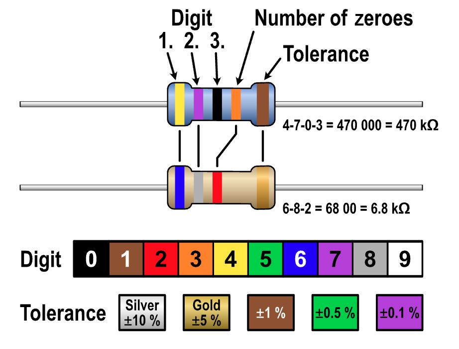 Figure 1. Resistor codes including the information of the resistances and tolerances. This file is made available under the Creative Commons CC0 1.0 Universal Public Domain Dedication via Wikimedia Commons.
The structure of a metal-film resistor is more involved than it may first appear. Figure 2 shows that a typical resistor includes a ceramic core, a thin resistive film, and often a helical cut to fine-tune the resistance value. The resistance depends primarily on the resistivity of the film, the geometry of the conducting path, and how precisely it can be trimmed during manufacturing. Each of these parameters — film thickness, width of the spiral cut, or even slight misalignments — carries a degree of uncertainty. Figure 3 illustrates, in concept, how variations in input parameters can lead to a distribution in resistance values. (Note: This is a simplified example for explanatory purposes.)
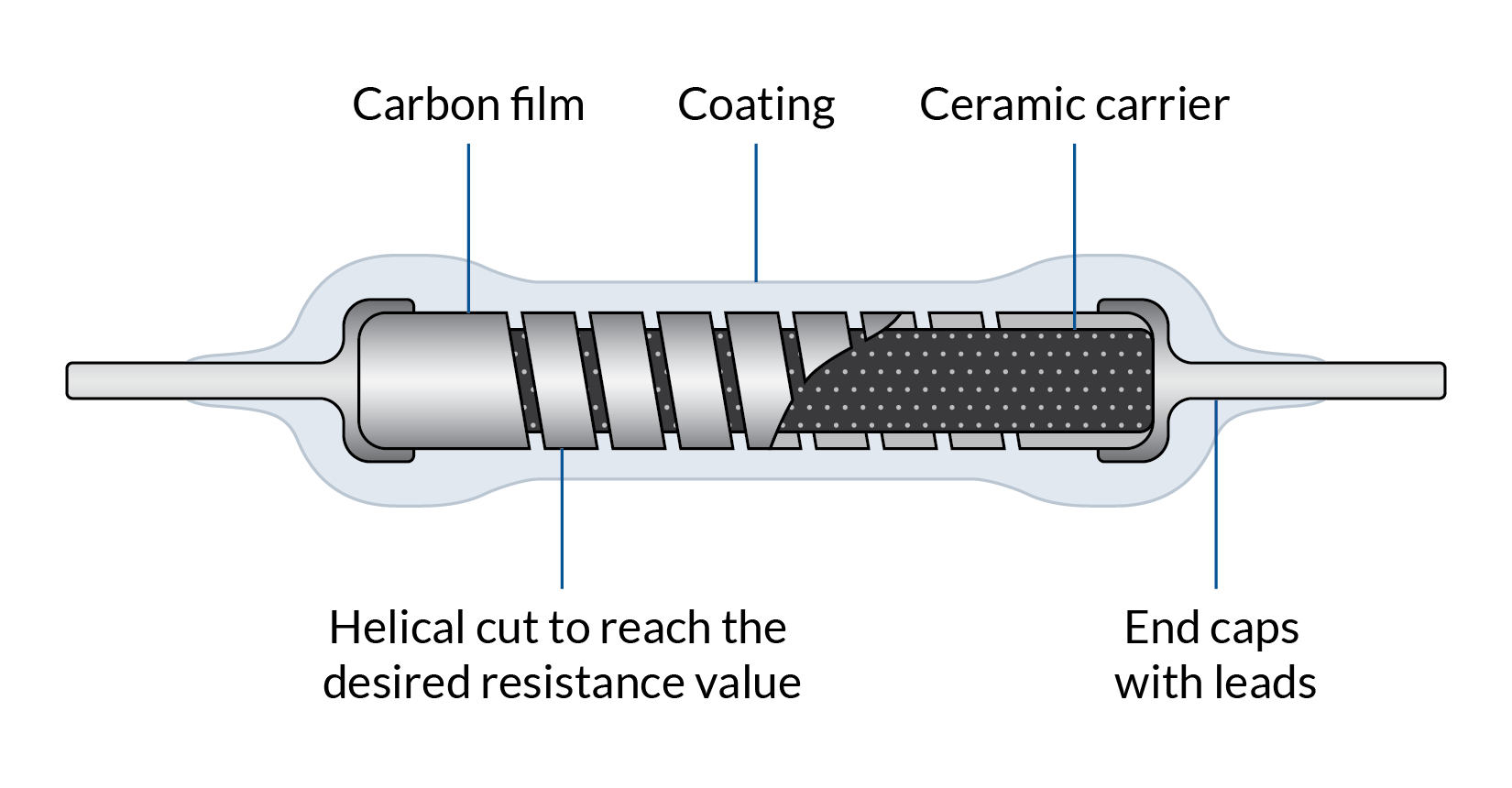 Figure 2. Metal film resistor structure and components.
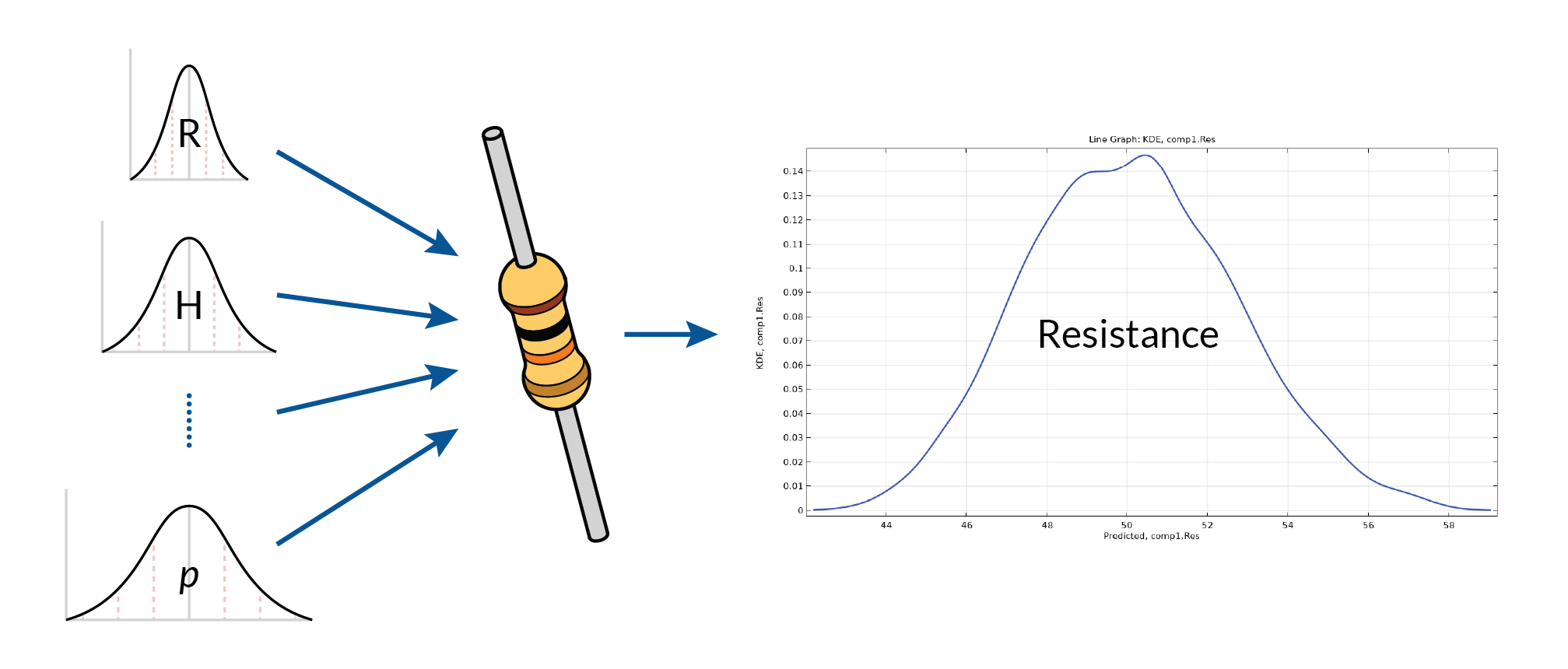 Figure 3. Illustration that depicts how the different distributions in the input parameters could affect the resistance distribution.
For manufacturers, maintaining tight control over resistor tolerances means finding the right balance between performance and cost. This involves minimizing variability in materials and processes — from the consistency of the resistive film to the precision of helical trimming. Even subtle shifts in manufacturing conditions, such as tool wear or temperature drift, can affect resistance. With uncertainty quantification, manufacturers can simulate how these small fluctuations impact performance and identify which production factors are worth optimizing to improve yield and product reliability.
For engineers integrating these resistors into circuits, the focus shifts to how parameter variability affects circuit behavior. Will a resistor that’s 5% off still allow the voltage divider to work as expected? What about a timing circuit relying on precise RC constants? UQ helps provide clear answers to these design questions by revealing the range and likelihood of different outcomes — all before building a prototype.
The Uncertainty Quantification Module
To explore this scenario further, we built a resistor model in the COMSOL Multiphysics® software using the Electric Currents interface, as shown in Figure 4. A voltage difference was applied across the two terminals, and the resistance was calculated from the power dissipation. Resistance was set as the quantity of interest (QoI), as V_0^2/\int qdV, where q is the volumetric loss density. We then performed a series of UQ studies using the Uncertainty Quantification Module.
Here’s what each type of study in the module is designed to do:
- Screening: Quickly identify what parameters matter on a resistance.
- Sensitivity: Quantify how much those parameters matter.
- Propagation: See the impact on the output. What would be the distribution in resistance based on all the distributions of the input parameter?
- Reliability: Can we trust the design? The probability for the resistance goes below or above a certain value.
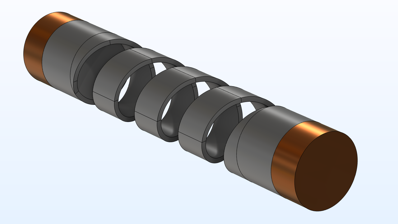 Figure 4. Resistor model in COMSOL Multiphysics.
Screening Analysis: Identifying the Key Parameters
The first UQ study performed is a screening analysis using the Morris one-at-a-time (MOAT) method. This study considers multiple input parameters with assumed distributions, mostly normal (Figure 5).
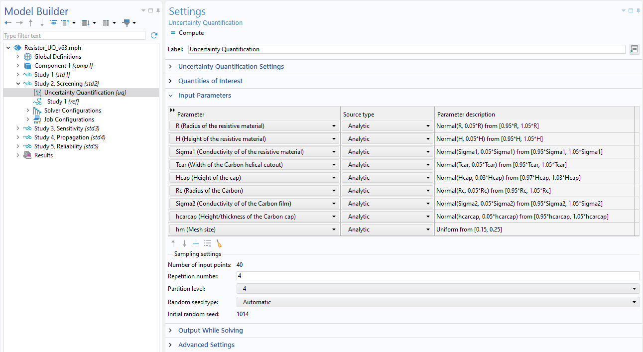 Figure 5. Input parameters.
Figure 6 shows the most influential parameters as the MOAT mean values; highlighting radius (R), height (H), conductivity (Sigma2), and etch width, or the width of the carbon helical cutout (Tcar). This aligns with theoretical expectations and enables us to streamline the following analyses by focusing only on these key variables, reducing computational cost.
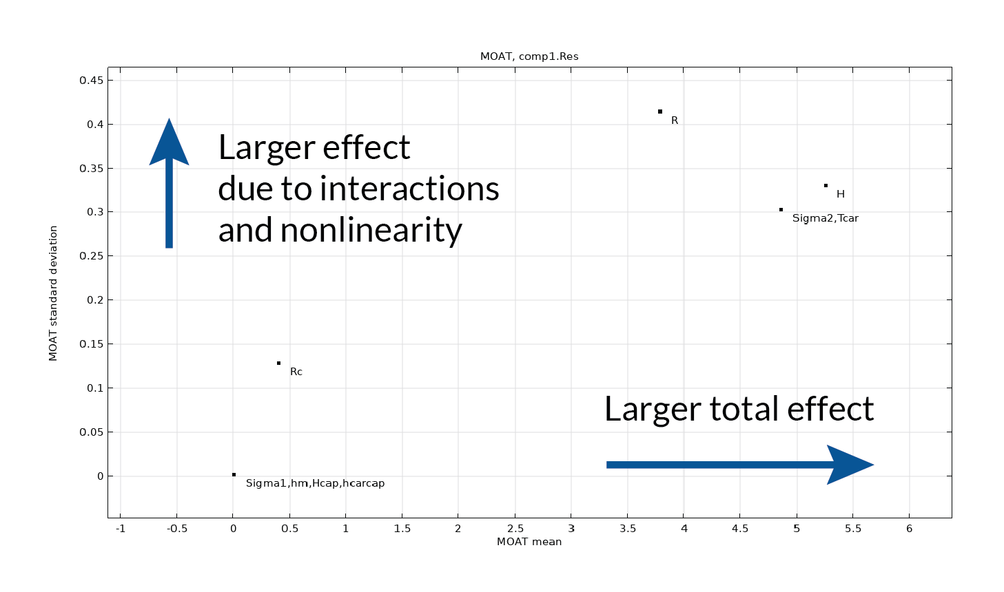 Figure 6. The MOAT mean is proportional to the total effect of a parameter on the QOI.
Sensitivity Analysis: Measuring the Impact
Next, we performed a sensitivity analysis using a sparse polynomial chaos expansion (PCE) surrogate model, which was automatically constructed to efficiently explore the input space. Figure 7 shows the Sobol indices, which quantify each parameter’s contribution to the resistance variance. The results indicate that height (H) is the most dominant factor, followed by conductivity (Sigma2) and etch width (Tcar).
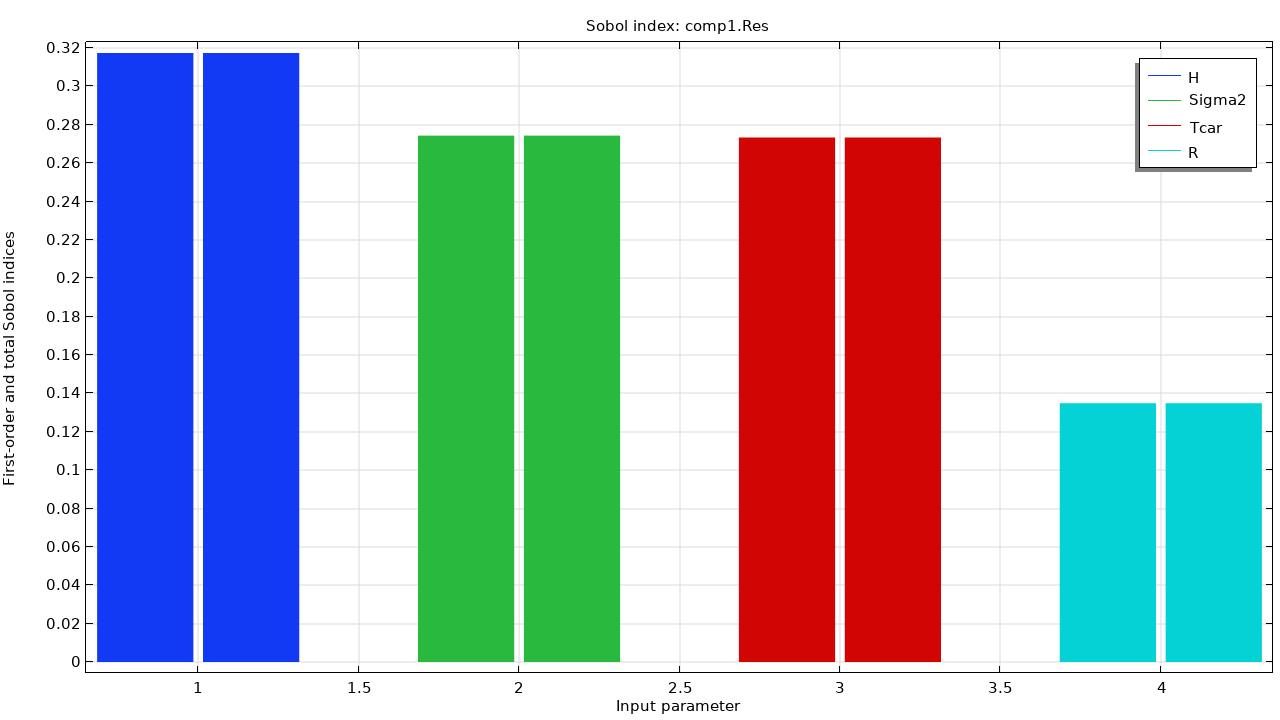 Figure 7. Sobol index vs. input parameter.
Uncertainty Propagation: Understanding Output Distribution
In the uncertainty propagation study, we sample the input parameter distributions and generate a kernel density estimation (KDE) plot (Figure 8). This plot displays the probability distribution of the resistance value. The result gives manufacturers a realistic view of how resistance might vary across production samples. The plot shows that the highest probability density occurs around a resistance value of 50. According to the QoI confidence interval table, the mean of the predicted resistance value is 50.099, and the standard deviation is 2.5821.
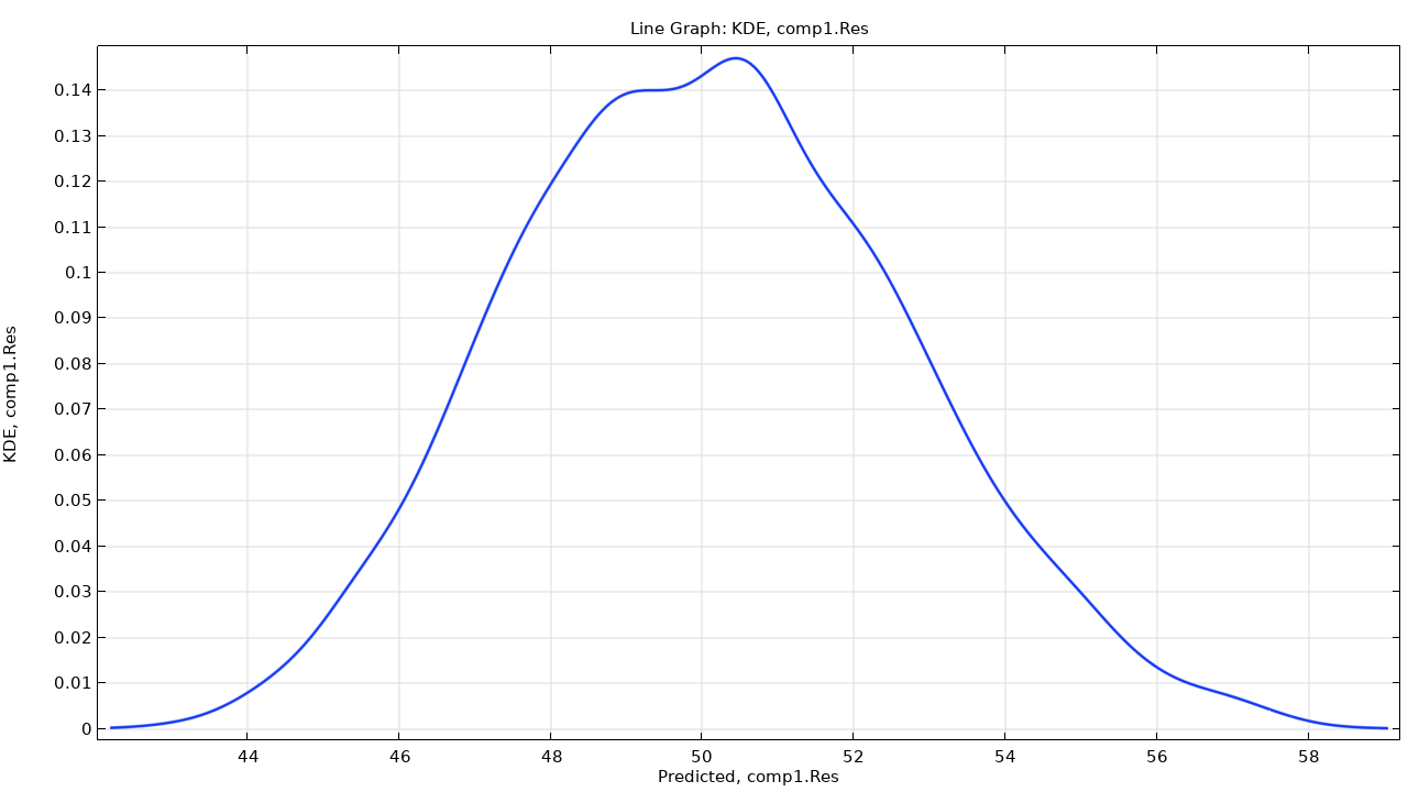 Figure 8. The kernel density estimation (KDE) plot.
Reliability Analysis: Quantifying Risk
Finally, a reliability analysis estimates the probability of resistance exceeding a set threshold, which is useful in any design with strict tolerances. Figure 9 shows the probability of the resistance crossing a defined value, helping quantify risk early in the design process. In this case, the probability with this condition will be about 0.19, or 19%.
Together, these four study types provide a comprehensive understanding of how input variability affects resistor performance, from identifying influential parameters to estimating failure probability.
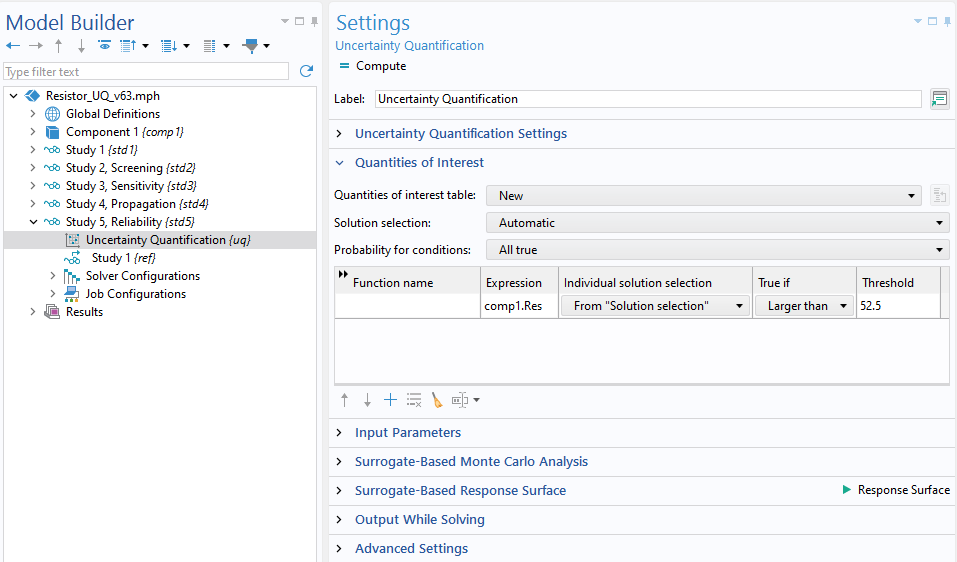 Figure 9. Probability of the conditions.
Final Thoughts: Using UQ in Resistor Design
Uncertainty quantification gives engineers and manufacturers the tools to understand how variations in materials, geometry, and processes affect performance. Whether you’re optimizing a resistor fabrication process or assessing the stability of a circuit design, the Uncertainty Quantification Module and COMSOL Multiphysics® can help you identify the most important variables, estimate output variation, and make data-driven decisions to balance reliability and cost.
Engineers designing with off-the-shelf resistors can also take advantage of resistance distribution data provided by manufacturers or obtained from measurements. Instead of treating resistance as a fixed value, they can use this distribution directly in a UQ study of their circuit. This allows for early-stage evaluation of design robustness: determining, for example, whether a given tolerance in a resistor will affect timing, gain, or signal thresholds — all before committing to hardware.
Next Steps
To get hands-on experience with the model presented here, click the button below.
- For a deeper dive, explore the Introduction to Uncertainty Quantification course, featuring practical, simulation-driven examples like a steel bracket model
- See a more advanced use case in this article on applying the Uncertainty Quantification Module to analyze frequency variation in a MEMS resonator
FIFA World Cup is a trademark or registered trademark of the Federation Internationale de Football Association.


Comments (0)