

Think about the first architects who designed a bridge above water. The design process likely included several trials and subsequent failures before they could safely allow people to cross the river. COMSOL Multiphysics and the Optimization Module would have helped make this process much simpler, if they had computers at the time, of course. Before we start to discuss building and optimizing bridges, let’s first identify the best design for a simple beam with the help of topology optimization.
A Simple Beam Case
In our structural steel beam example, both ends of the beam are on rollers, with an edge load acting on the top of the middle part. The beam’s dimensions are 6 m x 1 m x 0.5 m. In this case, we stay in the linear elastic domain and, due to the dimensions, we can use a 2D plane stress formulation. Note that there is a symmetry axis at x = 3 m.
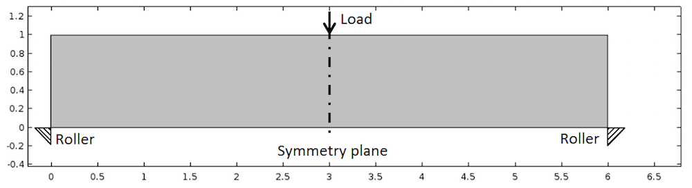
Geometry of the beam with loads and constraints.
Choosing the Right Optimization Type to Find a Structure’s Best Design
Using the beam geometry depicted above, we want to find the best compromise between the amount of material used and the stiffness of the beam. In order to do that we need to convert this into a mathematically formal language for optimization. Every optimization problem consists of finding the best design vector \alpha, such that the objective function F(\alpha) is minimal. Mathematically, this is written as \displaystyle \min_{\alpha} F(\alpha).
The design vector choice defines the type of optimization problem that is being solved:
- If \alpha is a set of parameters driving the geometry (e.g., length or height), we are talking about parametric optimization.
- If \alpha controls the exterior curves of the geometry, we are talking about shape optimization.
- If \alpha is a function determining whether a certain point of the geometry is void or solid, we are talking about topology optimization.
Topology optimization is applied when you have no idea of the best design structure. On the one hand, this method is more flexible than others because any shape can be obtained as a result. On the other hand, the result is not always directly feasible. As such, topology optimization is often used in the initial phase, providing guidelines for future design schemes.
In practice, we define an artificial density function \rho_{design}(X) , which is between 0 and 1 for each point X = \lbrace x,y \rbrace of the geometry. For a structural mechanics simulation, this function is used to build a penalized Young’s modulus:
where E_0 is the true Young’s modulus. Thus, \rho_{design}= 0 corresponds to a void part and \rho_{design}= 1 corresponds to a solid part.
As mentioned before, in regards to the objective function, we want to maximize the stiffness of the beam. For structural mechanics problems, maximizing the stiffness is the same as minimizing the compliance. In terms of energy, it is also equivalent to minimizing the total strain energy defined as:
Our topology optimization problem is thus written as:
Addressing Topology Optimization in COMSOL Multiphysics
Now that our optimization problem has been defined, we can set it up in COMSOL Multiphysics. In this blog post, we will not detail the solid mechanics portion of our simulation. There are, however, several tutorials from our Structural Mechanics Module that help showcase this element.
When adding the Optimization physics interface, it is possible to define a Control Variable Field on a domain. As a first discretization for \rho_{design}, we can select a constant element order. This means that we will have one value of \rho_{design} through all the mesh elements.
After this step is completed, a new Young’s modulus can be defined for the structural mechanics simulation, such as E(X)=\rho_{design} E_0.
As referenced above, the objective function is an integration over the domain. In the Optimization interface, we select Integral Objective. The elastic strain energy density is a predefined variable named solid.Ws. Thus, the objective can be easily defined as \int_\Omega Ws \ d\Omega.
Our discussion today will not focus on how optimization works in practice. Basically, the optimization solver begins with an initial guess and iterates on the design vector until the function objective has reached its minimum.
If we run our optimization problem, we get the results shown below.
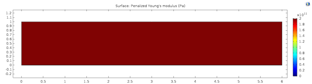
Results from the initial test.
The solution is trivial in order to maximize the stiffness. The optimal solution shows the full amount of the original material!
After this initial test, we can conclude that a mass constraint is necessary if we want to make the optimization algorithm select a design. With a constraint of 50 percent, this could be written as:
In COMSOL Multiphysics, a mass constraint can be included by adding an Integral Inequality Constraint. Additionally, the initial value for \rho_{design} needs to be set to 0.5 in order to respect this constraint at the initial state.
Let’s have a look at the results from this new problem, which are illustrated in the following animation.
Results with the addition of a mass constraint.
While this result is better, a problem remains: We have many areas with intermediate values for \rho_{design}. For the design, we only need to know if a given area is void or not. In order to get mostly 1 or 0 for the \rho_{design}, the intermediate values must be penalized. To do so, we can add an exponent p in the penalized Young’s modulus expression:
In practice, p is taken between 3 and 5. For instance, if p = 5 and \rho_{design}= 0.5, the penalized Young’s modulus will be 0.03125 E_0. The contribution for the mass constraint, meanwhile, will still be 0.5. As such, the optimization algorithm will try lending to 0 or 1 for the design vector.
With our new penalized Young’s modulus, we get the following result.
Results with the new penalized Young’s modulus.
A beam design has started to emerge! There is, however, a problematic checkerboard design, one that seems to be highly dependent upon the chosen mesh. In order to avoid the checkerboard design, we need to control the variations of \rho_{design} in space. One way to estimate variations of a variable field is to compute its derivative norm integrated on the whole domain:
A new question arises: How can we minimize both the variation of \rho_{design} and the total strain energy?
Since a scalar objective function is necessary, these objectives must be combined. We can think about adding them, but first, the two expressions need to be scaled to get values around 1. Concerning the stiffness objective, we simply divide by Ws0, which is the value of the total strain energy when \rho_{design} is constant. In regards to the regularization term, we can take the following scaling factor \frac{h_0 h_{max}}{A}, where h_{max} is the maximum mesh size, h_0 is the expected size of details in the solution, and A is the area of the design space. Our final optimization problem is now written as:
where the factor q controls the regularization weight.
Finally, the discretization of \rho_{design} needs to be changed to Lagrange linear elements to enable the computation of its derivative.
By solving this final problem, we obtain results that offer helpful insight as to the best design structure for the beam.
Results with regularization.
Such a design scheme can be seen at different scales in the real world, as illustrated in the bridge below.

A warren-type truss bridge. Image in the public domain, via Wikimedia Commons.
Designing a Bridge Above Water
Now that we have set up our topology optimization method, let’s move on to a slightly more complicated design space. We want to answer the question of how to design a bridge above water. To do so, a road zone in the geometry must be defined where the Young’s modulus is not penalized.
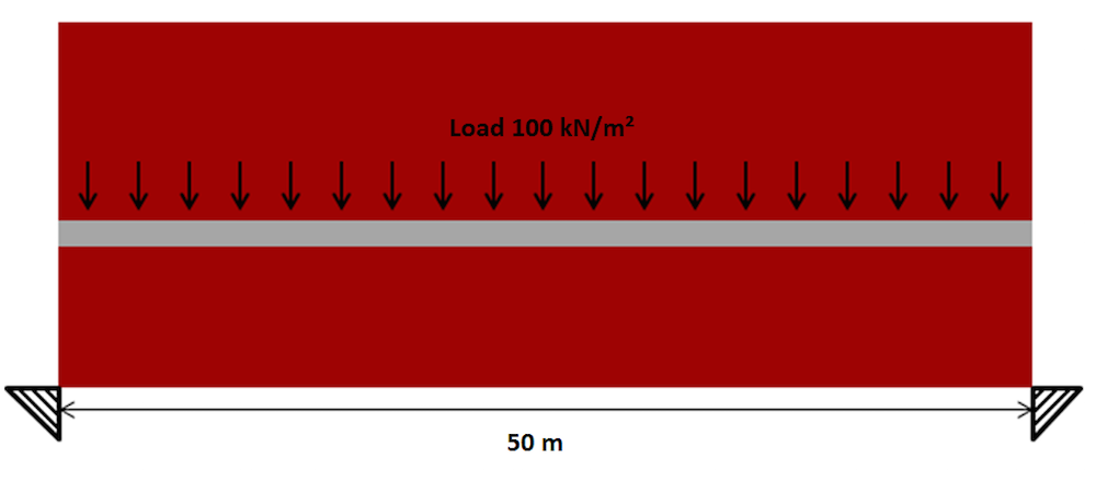
Design space for a through-arch bridge.
After a few iterations, we obtain a very good result for the through-arch bridge, one that is quite impressive. Such a result could provide architects with a solid understanding of the design that should be used for the bridge.
Topology optimization results for a through-arch bridge.
While the mathematical optimization algorithm had no guidelines on the particular design scheme, the result depicted above likely brings a real bridge design to mind. The Bayonne Bridge, shown below, is just one example among many others.

The Bayonne Bridge. Image in the public domain, via Wikimedia Commons.
It is important to note that this topology optimization method can be used in the exact same way for 3D cases. Applying the same bridge design question, the animation below shows a test in 3D for the design of a deck arch bridge.
3D topology optimization for a deck arch bridge.
Concluding Thoughts
Here, we have described the basics of using the topology optimization method for a structural mechanics analysis. To implement this method on your own, you can download the Topology Optimization of an MBB Beam tutorial from our Application Gallery.
While topology optimization may have initially been built for a mechanical design, the penalization method can also be applied to a large range of physics-based analyses in COMSOL Multiphysics. Our Minimizing the Flow Velocity in a Microchannel tutorial, for instance, provides an example of flow optimization.
References
- “Optimal shape design as a material distribution problem”, by M.P. Bendsøe.
- Topology Optimization: Theory, Methods, and Applications, by M.P. Bendsøe and O. Sigmund.


Comments (3)
Dustin Gerrard
March 2, 2016The topology optimization feature in COMSOL is very useful. I am having difficulty getting MMA to work with anything besides a stationary study. Is it possible to do MMA topology optimization with an eigenfrequency study? Or another study?
I want to change the frequency and quality factor based on the topology of a resonating device. In the book you reference by M.P. Bendsøe and O. Sigmund section 2.1 they describe topology optimization of a dynamic device.
René Christensen
October 25, 2017I know you asked this question a while back, but sure, MMA can be used e.g. in a harmonic study, see https://www.comsol.dk/blogs/how-to-use-acoustic-topology-optimization-in-your-simulation-studies/
Best regards
René Christensen, PhD
Trevor Munroe
March 17, 2019It would be nice to update this blog using the new density method in version 5.4.