

The COMSOL Multiphysics® software is often used to solve problems involving field solutions to partial differential equations (PDEs), but it also has the capability to solve ordinary differential equations (ODEs). For example, we can solve Newton’s second law for the motion of a satellite about a planet. Solving this equation on its own is quite straightforward, and you can combine this capability with the results presentation features of the software to make some very nice visualizations. Let’s learn more!
Computing Satellite Orbits
When modeling a satellite orbiting about Earth, we can start by writing the expression for the gravitational force experienced by an object:
where \phi is a potential function.
We will work in a Cartesian coordinate system centered at Earth. To account for the fact that Earth is slightly nonspherical, we use the following expression for the potential:
where \mu_{\oplus} is the standard gravitational parameter of Earth, r is the distance from the earth center to satellite, J_2 is the second term in the spherical harmonic expansion of the geopotential model of Earth, and P_2 is the second Legendre polynomial.
This second term in the potential accounts for the equatorial bulge of Earth and leads to precession of the satellite.
We can write an expression for this potential by using the legendre() function, one of the built-in mathematical functions within COMSOL Multiphysics. We could also use the built-in sum() operator to include higher-order terms in our potential function, but these are ignored here, since they are significantly smaller.
If we assume that there are only gravitational forces on the satellite, then the governing ordinary differential equation for the satellite position is:
Solving this equation requires initial conditions for position, \mathbf{ {x}}_0, and velocity \mathbf{\dot {x}}_0. The position of a satellite is typically given in terms of Keplerian orbital elements. For a general elliptical orbit, the eccentricity, \epsilon; semimajor axis, a; inclination, \epsilon; longitude of ascending node, \Omega; and argument of periapsis, \omega, define an ellipse. The true anomaly, \nu, defines the position along that ellipse at start time. The longitude of the ascending node, inclination, and argument of periapsis correspond to the Z-X-Z proper Euler angles, and we can use the Rotated System feature within COMSOL Multiphysics to help us along. Once this coordinate system has been defined, as shown below, it makes available a set of nine matrix components that can convert from and to this coordinate system.
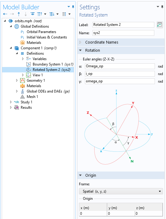
Screenshot of the Rotated System feature.
For example, if we assign the initial true anomaly, \nu_0, to be at the ascending node (when the satellite crosses the equator upward), then we can compute the initial position and velocity of the satellite in the orbital plane with just a bit more math. We can then use the components of the transformation matrix to get the initial positions in the global coordinate system, relative to the planet center. From that, we have the complete model definition and are ready to set up the ODE and solve it.
We can use the Global ODEs and DAEs interface and enter equations for the position in the global coordinate system, as shown in the screenshot below. Simply appending t to the variable being solved for will take the time derivative, and appending twice will take the second time derivative, so the expression X_stt is equivalent to the x-component of the acceleration vector. On the other hand, when dealing with expressions such as the gravitational potential, differentiation is done via the d() operator, so d(Potential,X_s) is the x-component of the force of gravity.
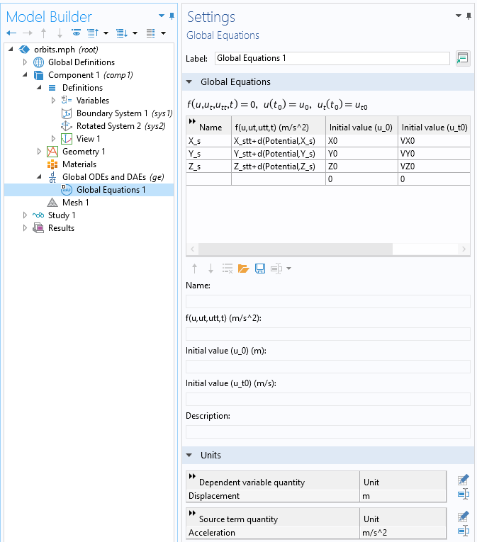
Solving an ODE for the satellite position about the planet center. Note how the units of the variable and the equation are set.
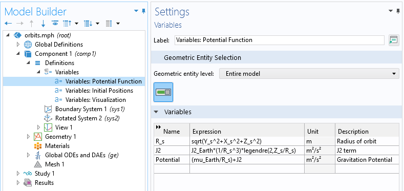
Solving the ODE for the position requires that expressions for the radius and gravitational potential are defined.
This set of equations and ODEs can be solved with any type of time-dependent solver, but regardless of the type, we will need to study the relative tolerance. Depending on our other modeling needs, the default BDF solver may be preferred, since it also allows for events: implicitly triggered changes in the equations during the transient solution.
Visualizing the Orbit
Once we solve the equations, we can plot the position and altitude of the satellite over time, and we might also like to make a visualization of the spacecraft in orbit. To that end, let’s next look at how to use some of the results visualization features, assuming that we have a CAD model representing our spacecraft, as shown below. A set of vectors, also shown, define the velocity-facing and nadir-facing directions. The cross-product of these two unit vectors is parallel to the normal of the orbital plane, as already described via the Rotated System feature.
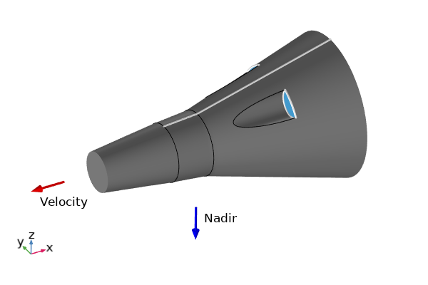
Simple CAD model of a spacecraft, along with vectors indicating how it is oriented in orbit relative to the CAD coordinate system.
Before plotting the spacecraft, the first thing that we want to do is create a visualization of Earth itself. For this, we use the Parameterized Surface dataset, which lets us write the expression of a sphere in terms of latitude and longitude.
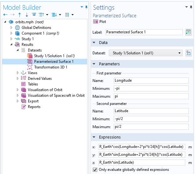
The Parameterized Surface dataset, which can be used to generate simple expression-based shapes such as spheres.
We can now use the Image plot feature to show an image mapped onto the dataset. Since the parameterized surface was set up in terms of latitude and longitude, an image using an equirectangular projection can be mapped onto it, as shown below.
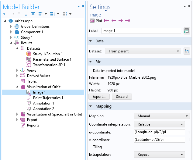
Image data plotted on a Parameterized Surface dataset.
Next, we might like to plot the orbit path. This can be done via the Point Trajectories plot type, which lets us enter trajectory data and the position of the spacecraft over time, and plot a line along its path. In addition, the Annotation plot type lets us evaluate and plot expressions that vary along the path.
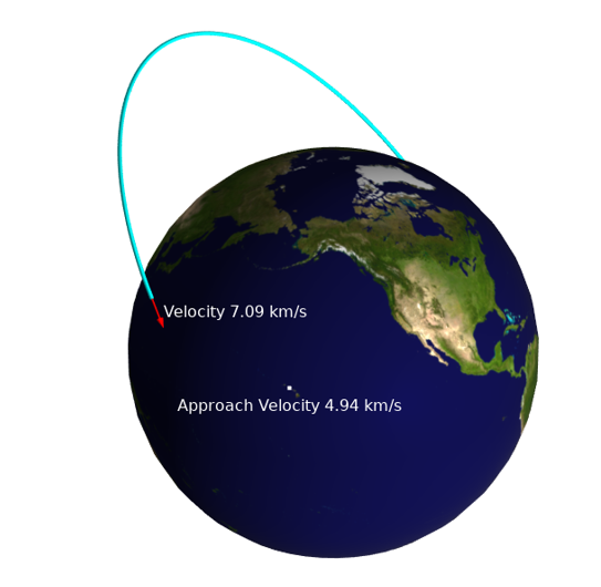
Using the point trajectories and annotation plots to visualize the satellite orbit and velocity information, as well as velocity relative to a ground station.
Finally, let us plot a scaled visualization of the spacecraft moving about Earth. This can be done via the Transformation 3D dataset, which allows for a general transformation type in terms of a set of base vectors that will appropriately scale and reorient the spacecraft about Earth, and a translation vector. In short, we just use the vectors defining the velocity and nadir directions, as well as the vector normal to the orbital plane, to reorient the spacecraft about Earth, as shown below.
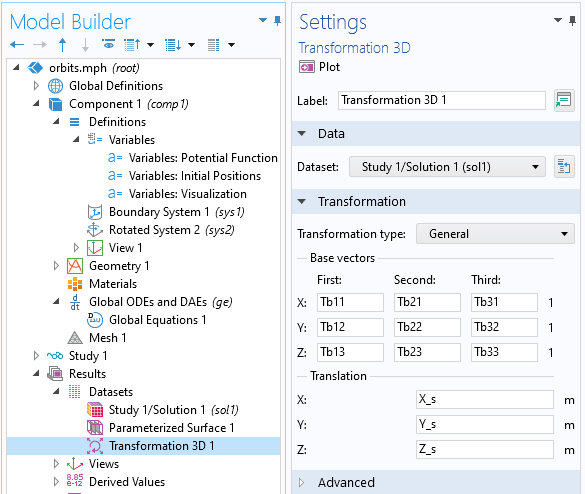
The Transformation 3D dataset can be used to reorient a dataset.
An animation of the spacecraft in orbit about the planet.
Closing Remarks
We have shown how to solve an ordinary differential equation that computes the motion of a satellite about the planet. It is quite simple to include more terms in the gravitational potential function to see their contributions, and the additional forces could be added to the ODE to account for atmospheric drag and other factors leading to orbital decay.
Alternatively, to simplify things, you could replace this ODE with an explicit equation for the position over time. Regardless of how we compute this trajectory, though, we can use the results functionality to create a variety of interesting and useful visualizations.
Try It Yourself
Try modeling a spacecraft in orbit yourself by clicking the button below, which will take you to the Application Gallery entry:
NASA Goddard Space Flight Center Image by Reto Stöckli (land surface, shallow water, clouds). Enhancements by Robert Simmon (ocean color, compositing, 3D globes, animation). Data and technical support: MODIS Land Group; MODIS Science Data Support Team; MODIS Atmosphere Group; MODIS Ocean Group. Additional data: USGS EROS Data Center (topography); USGS Terrestrial Remote Sensing Flagstaff Field Center (Antarctica); Defense Meteorological Satellite Program (city lights).

Comments (5)
Julian Anaya
March 14, 2022A very nice example, as usual, Walter. Just one comment, there is a typo in equation 2, u+ should be mu+ I think 😉
Walter Frei
March 14, 2022 COMSOL EmployeeThank you Julian, this should be updated now!
limbhaze na
March 29, 2022Visualization of the orbit motion of a satellite in space is an important step to carryout mission planning and design. In an environment of learning such visualization tools help the students to understand and appreciate the dynamical motion. The purpose of this study was to present, first, the simulation of the satellite orbit analysis based on data collected from NASA/Norad two line element files. The analysis includes orbit determination and prediction of satellite position/velocity, orbit eclipse and ground trace and so on. Second the application of this simulation to design the Low Earth Orbit (LEO) satellite power subsystem. The intention of this simulation was to create a Graphical User Interface (GUI) which consists of menus, push buttons, text boxes, plots and other interface devices that allow the GUI user to immediately see the impact of various changes.
Joseph Zarrabi
December 16, 2022It is a nice simulation by Walter. Is it possible that to get the step-by-step pdf instructions how to set this up? Usually in COMSOL, when a COMSOL solution is provided then there is a pdf file showing how to set the model using step-by-step instructions.
Walter Frei
December 16, 2022 COMSOL EmployeeHello Joseph,
Regarding this example, we now have functionality within the Heat Transfer Module to address orbit modeling. For an overview, see: https://www.comsol.com/blogs/computing-orbital-heat-loads-with-comsol-multiphysics/
There are a set of examples available, with step-by-step instructions:
https://www.comsol.com/model/orbit-calculation-109301
https://www.comsol.com/model/orbit-thermal-loads-109801
https://www.comsol.com/model/spacecraft-thermal-analysis-109811
We would say that the contents of this blog are now superseded by the new functionality, although there might still be some general educational interest in the example and model presented here.