
Suppose you are recreating a model, perhaps from one of the Application Libraries that are included with the COMSOL Multiphysics® software and its add-on products. You might be doing so to learn about how to set up a model with a specific functionality. However, the version that you created does not provide the same results as the original. How do you find the differences between the two versions of the model?
Using the Model File Comparison Tool
Any time you are interested in comparing two COMSOL Multiphysics model files, you can use the Compare tool to compare the current model in the COMSOL Desktop® with any other COMSOL Multiphysics model file available on your file system (called the Remote file in the Compare tool) . By comparing model files, you can:
- Identify and correct errors in the current model
- Document and check differences between two versions of a model under development
- Provide the differences between the two model files as an XML file for further processing
The Compare button is available on the Developer toolbar.

![]()
The Compare button is the rightmost button on the Developer toolbar for the Windows® operating system (top) and for the Linux® operating system and macOS (bottom).
When you click the Compare button, a Select Application window opens, where you can choose any COMSOL Multiphysics file (MPH file) from the file system. Then, click Open to open that file and perform the comparison. The comparison appears in a Comparison Result window in the COMSOL Desktop®.

The Comparison Result window, with a list of differences between the open local file and a remote file.
Click the Detailed Comparison of Selected Attribute button or double-click the row with the attribute to open a Compare Attribute window with more detailed information about the comparison.

The Compare Attribute window provides a more detailed view of the differences between the values of an attribute; in this case, differences in which boundaries are selected.
Typical Differences Between Two Models
When creating or recreating a COMSOL Multiphysics model, there are a couple of mistakes that can make the results of the model differ from what you expected.
For instance, the model can include a value of some source, flux, material property, or other input that was not the intended value. This can be due to a small mistake, such as a misplaced decimal point, for example. Depending on the usage and impact of the changed value, it can have a dramatic effect on the results.
Another possible error is selecting the incorrect boundary when determining where a boundary condition is active. The wrong set of boundaries can be selected by mistake, or, if the geometric entity numbers are entered from some model documentation, there can be a mismatch between the numbering of the actual geometric components in the current model and the previous model. Such a mismatch could be caused by some changes in how the geometry in the model was created. It can also be the case that the selection for an added boundary condition or domain source is empty, or not active for any geometric entity. In that case, the node in the model tree shows a warning, and a tooltip appears with the message Selection is empty to help you identify such physics nodes.
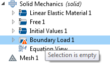
The tooltip and warning for an added physics node with no selection.
For these cases — except perhaps the case of an empty selection, which should be easy to spot — the comparison tool is very useful in finding the exact differences between two supposedly identical COMSOL Multiphysics models. The examples below, using the Automotive Muffler model from the COMSOL Multiphysics Application Library, show how you can use this tool to find such differences.
The model contains a simulation of the pressure wave propagation in a muffler for a combustion engine. The following plots show the solution from the model in the Application Library and from two model files that recreate the example but use an incorrect inlet pressure amplitude and outlet boundary selection, respectively.


The solution for the acoustic pressure for the original model from the Application Library (top left), for the model with the incorrect inlet pressure (middle), and for the model with the incorrect selection of outlet boundaries (right).
Unintentionally Changed Values
Let’s say that your finger slips on your keyboard when entering the value for the parameter p0 for the inlet pressure amplitude, so that the value becomes 11 Pa instead of 1 Pa, as it is in the Application Library version of the model. As expected, the resulting pressure becomes 11 times higher, which the middle plot above shows. Using the comparison tool, the Comparison Result window shows the following difference:
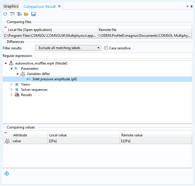
The Comparison Result window, showing the difference in the local and remote values for the inlet pressure amplitude.
In the Differences section above, there are other differences in the exact camera positions (under Views) and the timestamps for the solvers (under Solver sequences), which are natural differences that you can ignore.
Under Results, there are differences in the plot data ranges, which is an effect of the changes in the solution. If you had some prior knowledge or hunch that the difference had to do with pressure, then a filtered view of the comparison result shows only the change in the inlet pressure amplitude:
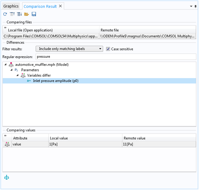
A filtered view of the differences in the Comparison Result window, showing only the difference for the inlet pressure amplitude.
Correcting the value of the parameter for the inlet pressure amplitude from 11 Pa to 1 Pa and then re-solving the model results in a solution that is identical to that of the Application Library model.
Different Selection of Boundaries
In this scenario, the selection of the outlet boundary is incorrect. Perhaps the top boundary of the exit pipe was enclosed by mistake when making the selection in the Graphics window. Such an incorrect selection affects the solution so that the acoustic pressure changes slightly and the pressure isosurfaces have a different shape and location, as the right plot above shows. Using the comparison tool, the Comparison Result window shows the following difference:
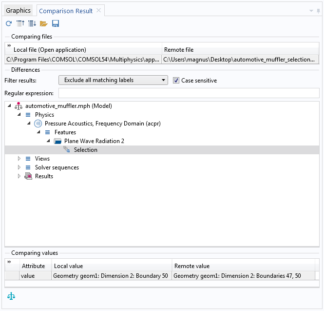
The Comparison Result window, showing the difference in the local and remote value for the selection of the Plane Wave Radiation boundary condition, representing the outlet.
In the Differences section above, there are other differences that you can ignore, just like in the previous comparison. If you think that the difference has to do with some selection, then a filtered view of the comparison result shows only the change in the selection of outlet boundaries:

A filtered view of the differences in the Comparison Result window, showing only the difference for the selection of outlet boundaries.
By changing the selection for the outlet to include only boundary 50 and then re-solving the model, we get a solution that is identical to the Application Library model.
Conclusions and Next Steps
In this blog post, we have demonstrated how the comparison tool in COMSOL Multiphysics can help you pinpoint differences between two COMSOL Multiphysics model files. For two examples of common modeling mistakes, the comparison tool finds the differences that make the solutions differ from the expected solution. It is easy to correct these types of mistakes so that the recreated model provides the correct solutions.
Browse the Application Gallery to try recreating — and comparing — one of the tutorial models:
Read this blog post on how to find interesting examples in the Application Libraries: How to Search for a Specific COMSOL Multiphysics® Application
Linux is a registered trademark of Linus Torvalds in the U.S. and other countries. macOS is a trademark of Apple Inc., in the U.S. and other countries. Microsoft and Windows are either registered trademarks or trademarks of Microsoft Corporation in the United States and/or other countries.


Comments (2)
Ivar KJELBERG
April 16, 2019Thanks Magnus,
This comparison tool gives us now the required insights to improve our quality assurance for our models.
Models are made so quickly, but become as rapidly so complex, impossible without this to check for model coherence.
Hours gained in on quality check list, and more time to study physics, the fun of it 🙂
Sincerely
Ivar
Magnus Ringh
April 16, 2019 COMSOL EmployeeThanks for the kind words Ivar! I’m glad that you like this functionality.
Best regards,
Magnus Ringh, COMSOL