
In applications such as power transfer and consumer electronics, it may be critical to model electromagnetic heating of materials that are nonlinear in temperature; that is, the material’s electrical conductivity and thermal conductivity vary with temperature. When modeling these nonlinearities, even an experienced analyst can sometimes get quite unexpected results due to the combination of the nonlinear material properties, boundary conditions, and geometry. Let’s find out why this is in terms of a very simple example.
Understanding Ohm’s Law and Resistive Heating
One of the first physical laws that we learn as engineers is Ohm’s law: The current through a device equals the applied voltage difference divided by the device electrical resistance, or I = V/Re, where the electrical resistance, Re, is a function of the device geometry and material’s electrical conductivity.
Shortly after learning that law, we probably also learned about the dissipated power within the device, which equals the current times the voltage difference, or Q = IV, which we could also write as Q = I2Re or Q = V2/Re. Maybe a little bit later in our studies, we also learned about thermal conductivity and equivalent device thermal resistance, Rt, which let us compute, in a lumped sense, the rise in temperature of a device via ΔT = QRt relative to ambient conditions. We can then determine the absolute device temperature using T = T_{ambient} + QR_t.
We start our discussion from this point and consider a completely lumped model of a device. (Yes, we’re starting so simple that we don’t even need to use the COMSOL Multiphysics® software for this part!) Let’s consider a lumped device with electrical resistance of Re = 1 Ω and thermal resistance of Rt = 1 K/W. We can drive this device with either a constant voltage and compute the temperature as T = T_{ambient} + (V^2 / R_e) R_t or drive it via constant current where the peak temperature is T = T_{ambient} + I^2 R_e R_t.
We choose an ambient temperature of 300 K, or 27°C, which is about room temperature. Let’s now plot out the device lumped temperature as a function of increasing voltage (from 0 to 10 V) and current (from 0 to 10 A), as shown in the image below. Unsurprisingly, we see a quadratic increase in temperature.
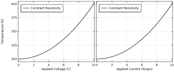
Device temperature as a function of applied voltage (left) and applied current (right), assuming constant properties.
We might think that we can use the curve to predict a wider range of operating conditions. Suppose we want to drive the device up to its failure temperature, where the material melts or vaporizes. Let’s say that this material will vaporize when its temperature gets up to 700 K (427°C). Based on this curve, some simple math would indicate that the maximum voltage is 20 V and the maximum current is 20 A, but this is quite wrong!
Introducing Material Nonlinearities into the Simple Lumped Model
At this point, you’re probably ready to point out the simple mistake that we’ve made: Electrical resistance is not constant with temperature. For most metals, the electrical conductivity goes down with an increasing temperature and since resistivity is the inverse of conductivity, the device resistivity goes up. So, let’s introduce a temperature dependence for the resistivity:
This is known as a linearized resistivity model, where ρ0 is the reference resistivity at T^e_0, the reference temperature, and αe is the temperature coefficient of electrical resistivity.
Let’s choose ρ0 = 1 Ω, T^e_0 = 300 K, and αe = 1/200 K. Now, the resistance is 1 Ω at a device temperature of 300 K and 2 Ω at a temperature rise of 200 K above the set temperature. The equations for lumped temperature as a function of voltage and current now become:
and
These equations are a bit more complicated (the first is a quadratic equation in terms of T) but still possible to solve by hand. The plots of temperature as a function of increasing voltage and current are displayed below.
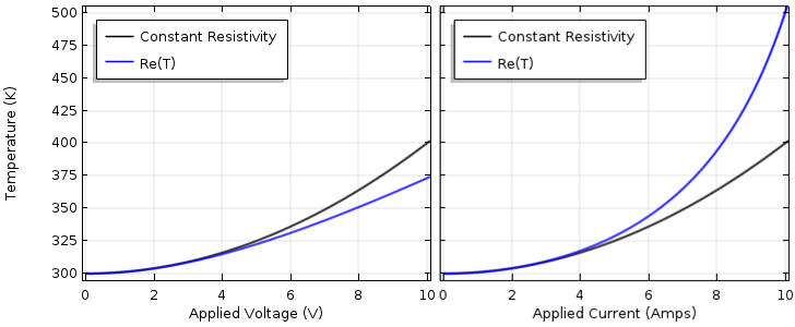
Device temperature as a function of applied voltage (left) and applied current (right) with the electrical resistivity as a function of temperature.
For the voltage-driven problem, as the temperature rises, the resistance rises. Since the resistance occurs in the denominator of the temperature expression, higher resistance lowers the temperature and we see that the temperature will be lower than that for the constant resistivity case. If we drive the device with constant current, the temperature-dependent resistance appears in the numerator. As we increase the current, the resistive heating will be higher than that for the linear material case.
We might be tempted at this point to compute the maximum voltage or current that this device can sustain, but you are probably already realizing the second mistake we’ve made: We also need to incorporate the temperature dependence of the thermal resistance. For metals, it’s reasonable to assume that the electrical and thermal conductivity will show the same trends. Thus, let’s use a nonlinear expression that is similar to what we used before:
Now, our voltage-driven and current-driven equations for temperature become:
and
Although only slightly different from before, these nonlinear equations are now quite a bit more difficult to solve. Simulation software is starting to look more attractive! Once we do solve these equations (let’s set r0 = 1 K/W, αt = 1/400 K, and T^t_0 = 300 K), we can plot the device temperature, as shown below.
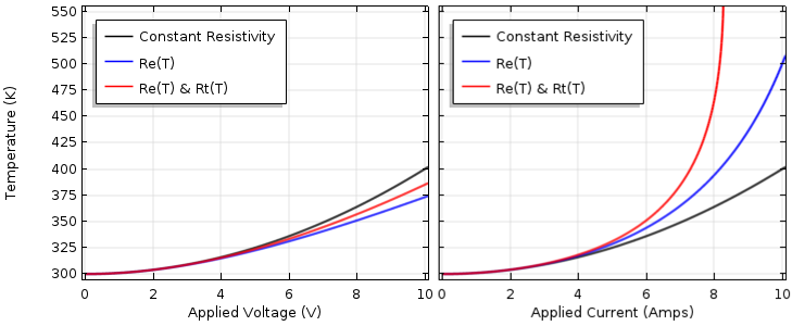
Device temperature as a function of applied voltage (left) and applied current (right) with the electrical and thermal resistivity as a function of temperature.
Observe that for the current-driven case, the temperature rises asymptotically. Since both the electrical and the thermal resistance increase with an increasing temperature, the device temperature rises very sharply as the current is increased. As the temperature rises to infinity, the problem becomes unsolvable. This is actually entirely expected; in fact, this is how your basic car fuse works. Now, if we were solving this problem in COMSOL Multiphysics, we could also solve this as a transient model (incorporating the thermal mass due to the device density and specific heat) and predict the time that it takes for the device temperature to rise to its failure point.
Things are luckily a bit simpler for the voltage-driven case. Here, we also see a predictable behavior: The rising thermal resistivity drives the temperature higher than when we only considered a temperature-dependent electrical conductivity. Now, the interesting point here is the temperature is still lower than for the constant resistivity case. This also sometimes confuses people, but just keep in mind that one of these nonlinearities is driving the temperature down while the other is driving the temperature up. In general, for a more complicated model (such as one you would build in COMSOL Multiphysics), you don’t know which nonlinearity will predominate.
What other mistake might we have made here? We have used a positive temperature coefficient of thermal resistivity. This is certainly true for most metals, but it turns out that the opposite is true for some insulators, glass being a common example. Usually, the total device thermal resistance is mostly a function of the insulators rather than the electrically conductive domains. In addition, the device’s thermal resistance should incorporate the effects of the cooling to the surrounding ambient environment. So, the effects of free convection (which increases with the temperature difference) and radiation (which has a fourth-order dependence on temperature difference) could also be lumped into this single thermal resistance. For now, though, let’s keep the problem (relatively) simple and just switch the sign of the temperature coefficient of thermal resistivity, αt = -1/400 K, and directly compare the voltage- and current-driven cases for driving voltage up to 100 V and current up to 100 A.
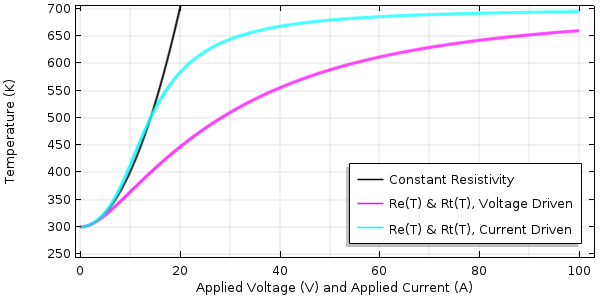
Device temperature as a function of applied voltage (pink) and applied current (blue) with a negative temperature coefficient of thermal resistivity.
We now see some results that are quite different. Observe that for both the voltage- and current-driven cases, the temperature increases approximately quadratically at low loads, but at higher loads, the temperature increase starts to flatten out due to the decreasing thermal resistivity. The slope, although always positive, decreases in magnitude. The current-driven case starts to asymptotically approach T = 700 K, but the voltage-driven case stays significantly below the failure temperature.
This is an important result and highlights another common mistake. The nonlinear material models we used here for electrical and thermal resistivity are approximations that start to become invalid if we get too close to 700 K. If we anticipate operating in this regime, we should go back to the literature and find a more sophisticated material model. Although our existing nonlinear material models did solve, we always need to check that they are still valid at the computed operating temperature. Of course, if we are not close to these operating conditions, we can use the linearized resistivity model (one of the built-in material models within COMSOL Multiphysics). Then, our model will be valid.
We can hopefully now see from all of this data that the temperature has a very complicated relationship with respect to the driving voltage or current. When nonlinear materials are considered, the temperature might be higher or lower than when using constant properties, and the slope of the temperature response can switch from quite steep to quite shallow just based on the operating conditions.
Have these results thoroughly confused you yet? What if we went back and changed one of the coefficients in the resistance expressions? Certain materials have negative temperature coefficients of electrical and thermal resistivity. What if we used an even more complicated nonlinearity? Would you feel confident in saying anything about the expected temperature variations in even this simple lumped device case, or would you rather check it against a rigorous calculation?
Concluding Thoughts on Common Pitfalls in Electrothermal Analysis
What about the case of a real-world device? One that has a combination of many different materials, different electrical and thermal conductivities as a function of temperature, and complex shapes? Would you model this under steady-state conditions only or in the time domain, to find out how long it takes for the temperature to rise? Maybe — in fact, most likely — there will also be nonlinear boundary conditions such as radiation and free convection that we don’t want to approximate via a single lumped thermal resistance. What can you expect then? Almost anything! And how do you analyze it? Well, with COMSOL Multiphysics, of course!
Next Step
Evaluate how COMSOL Multiphysics can help you meet your multiphysics modeling and analysis goals. Contact us via the button below.


Comments (1)
Ivar KJELBERG
April 18, 2018Hello Walter,
And what i you add some porous heating media with humid air and perhaps some other solvent, flowing through it, as you find in many industrial devices, even more fun again with COMSOL Multiphysics, the only issue: VV&C (the Validation, Verification and Calibration process) becomes more and more difficult, so you tend to deal with partial models and partial validations.
I was thought once by a PA/QA expert, he was Belgian and obviously had some reminders from their Africa time : “If you want to digest an Elephant, start to chop it down to handlebar sizes”.
And that is really easy in COMSOL: you build your model by steps, adding physics one by one and if possible, validate your step-wise construction of the full model.
Thanks for an instructive Blog
Sincerely,
Ivar