General Blog Posts

Intro to the What, Why, and How of Shared Memory Computing
A couple of weeks ago, we published the first blog post in a Hybrid Modeling series, about hybrid parallel computing and how it helps COMSOL Multiphysics model faster. Today, we are going to briefly discuss one of the building blocks that make up the hybrid version, namely shared memory computing. Before that, we need to consider what it means that an “application is running in parallel”. You will also learn when and how to use shared memory with COMSOL.
Size Parameters for Free Tetrahedral Meshing in COMSOL Multiphysics
COMSOL Multiphysics® has 9 built-in size parameter sets when meshing. In this blog post, we’ll discuss size parameters for 1 of these sets: free tetrahedral meshing.
Overview of Integration Methods in Space and Time
Integration is an important mathematical tool for numerical simulations. For example, partial differential equations are usually derived from integral balance equations.
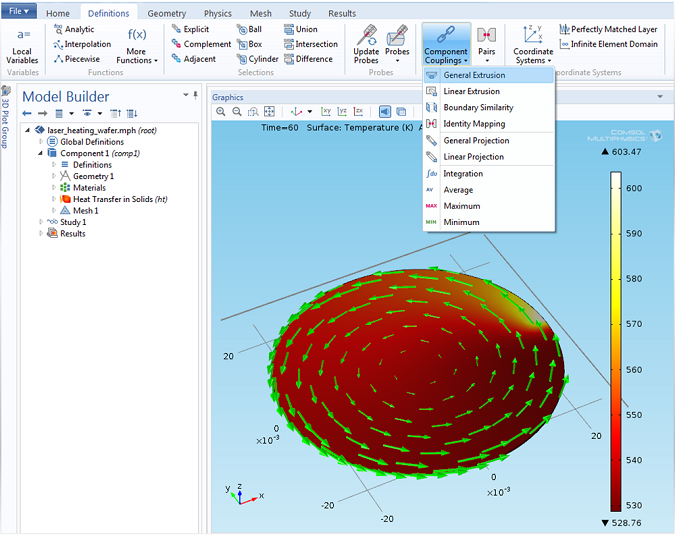
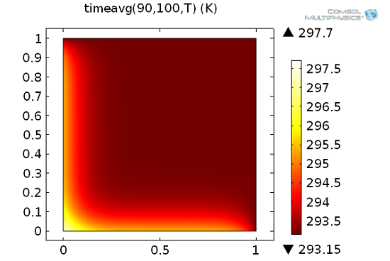
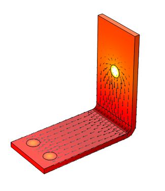
Using the General Extrusion Coupling Operator in COMSOL: Dynamic Probe
Consider a laser heating example with a moving heat source (laser) and moving geometry. How can you use the General Extrusion coupling operator to probe a solution at a point in the geometry?
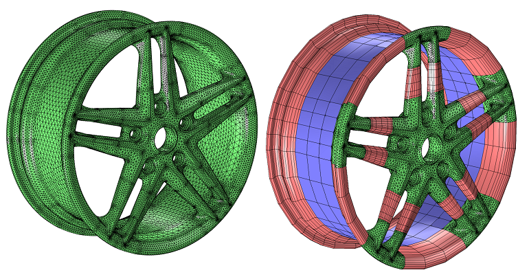
Hybrid Parallel Computing Speeds Up Physics Simulations
Remember 20 years ago, when the TOP500 list was dominated by vector processing supercomputers equipped with up to a thousand processing units? Let’s take a walk through history to the future.
Solving Algebraic Field Equations
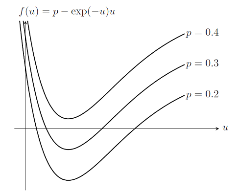
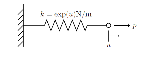
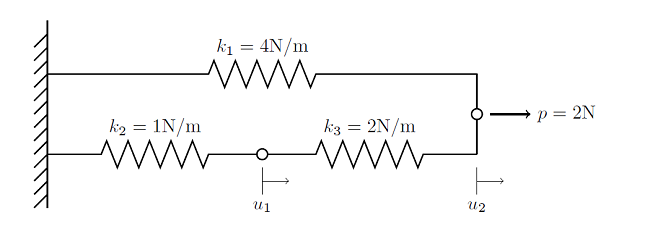
COMSOL Multiphysics® is commonly used to solve PDEs, ODEs, and initial value problems. However, did you know that you can also solve algebraic and even transcendental equations?
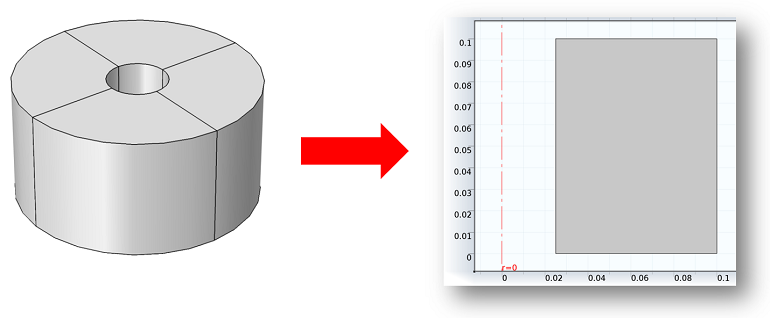
Visualization for 2D Axisymmetric Electromagnetics Models
Today we’ll look at how to make 3D plots of vector fields that are computed using the 2D axisymmetric formulation found in the Electromagnetic Waves, Frequency Domain interface within the RF and Wave Optics modules.

Using Adaptive Meshing for Local Solution Improvement
One of the perennial questions in finite element modeling is how to choose a mesh. We want a fine enough mesh to give accurate answers, but not too fine, as that would lead to an impractical solution time. As we’ve discussed previously, adaptive mesh refinement lets the software improve the mesh, and by default it will minimize the overall error in the model. However, we often are only interested in accurate results over some subset of the entire model space. […]
Learning to Solve Multiphysics Problems Effectively
One of the questions we get asked often is how to learn to solve multiphysics problems effectively. Over the last several weeks, I’ve been writing a series of blog posts addressing the core functionality of the COMSOL Multiphysics software. These posts are designed to give you an understanding of the key concepts behind developing accurate multiphysics models efficiently. Today, I’ll review the series as a whole.
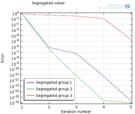
Improving Convergence of Multiphysics Problems
In our previous blog entry, we introduced the Fully Coupled and the Segregated algorithms used for solving steady-state multiphysics problems in COMSOL. Here, we will examine techniques for accelerating the convergence of these two methods.
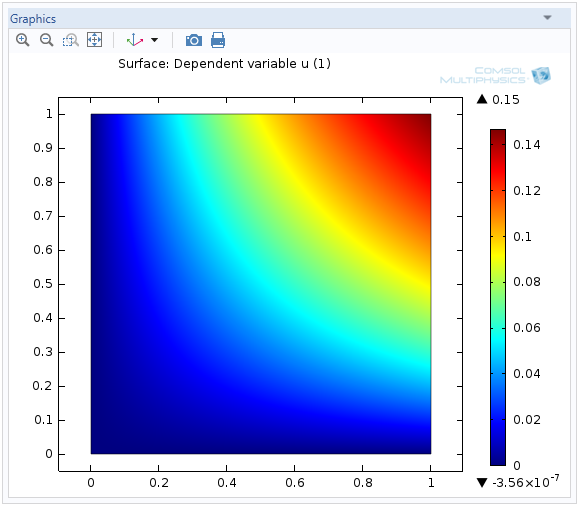
Simulating Viscous Fingering Using Equation-Based Modeling
A prospective user of COMSOL approached me about modeling viscous fingering, which is an effect seen in porous media flow. He hadn’t found a satisfying solution elsewhere, so he turned to COMSOL. I’d like to share with you some of my insight on how to go from idea to model to simulation by taking a “do-it-yourself approach” and utilizing the equation-based modeling capabilities of COMSOL Multiphysics.
Solving Multiphysics Problems
Here we introduce the two classes of algorithms used to solve multiphysics finite element problems in COMSOL Multiphysics. So far, we’ve learned how to mesh and solve linear and nonlinear single-physics finite element problems, but have not yet considered what happens when there are multiple different interdependent physics being solved within the same domain.
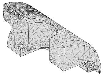
Meshing Considerations for Nonlinear Static Finite Element Problems
As part of our solver blog series we have discussed solving nonlinear static finite element problems, load ramping for improving convergence of nonlinear problems, and nonlinearity ramping for improving convergence of nonlinear problems. We have also introduced meshing considerations for linear static problems, as well as how to identify singularities and what to do about them when meshing. Building on these topics, we will now address how to prepare your mesh for efficiently solving nonlinear finite element problems.
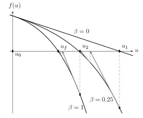
Nonlinearity Ramping for Improving Convergence of Nonlinear Problems
As we saw in “Load Ramping of Nonlinear Problems“, we can use the continuation method to ramp the loads on a problem up from an unloaded case where we know the solution. This algorithm was also useful for understanding what happens near a failure load. However, load ramping will not work in all cases, or may be inefficient. In this posting, we introduce the idea of ramping the nonlinearities in the problem to improve convergence.
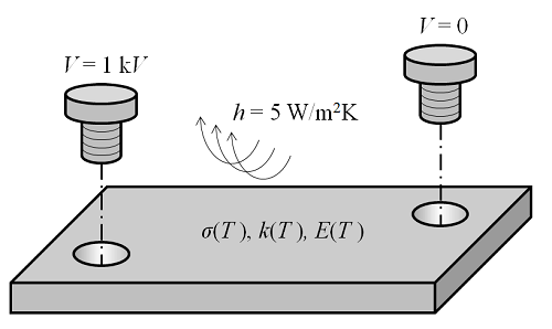
Dedicated Multiphysics Node Introduced in COMSOL 4.4
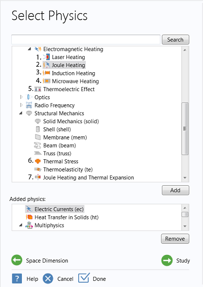
To make it easier and more transparent to define models involving multiple physics phenomena in COMSOL, a separate Multiphysics node has been added as a new feature in COMSOL version 4.4. The Multiphysics node gives you control over the couplings for thermal stress and electromagnetic thermal effects involved in your models. Future versions will include further multiphysics couplings through the Multiphysics node in addition to the multiphysics couplings methods already available since previous versions.
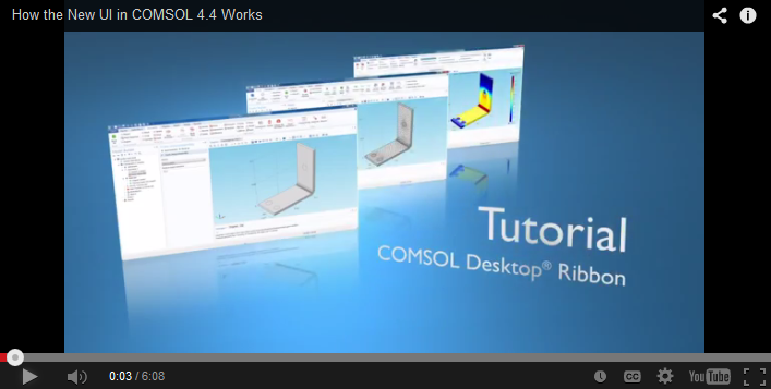
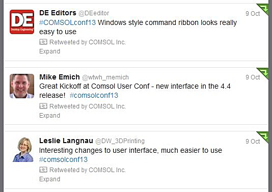
Video Tutorial: Introducing the New User Interface in COMSOL 4.4
Each COMSOL release aims to create a better modeling experience for our users, usually in the form of new add-on modules and new functionality in existing products. COMSOL 4.4 brings you all that, but it also includes another significant change: a brand new user interface (UI). The new UI contains a ribbon at the top of the interface (for our Windows® users) to make your modeling easier and faster. The ribbon gives you direct access to the functions you would […]
Load Ramping of Nonlinear Problems
As we saw previously in the blog entry on Solving Nonlinear Static Finite Element Problems, not all nonlinear problems will be solvable via the damped Newton-Raphson method. In particular, choosing an improper initial condition or setting up a problem without a solution will simply cause the nonlinear solver to continue iterating without converging. Here we introduce a more robust approach to solving nonlinear problems.
Solving Nonlinear Static Finite Element Problems
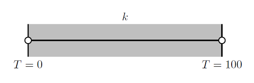
Here, we begin an overview of the algorithms used for solving nonlinear static finite element problems. This information is presented in the context of a very simple 1D finite element problem, and builds upon our previous entry on Solving Linear Static Finite Element Models.
Solutions to Linear Systems of Equations: Direct and Iterative Solvers
In this blog post we introduce the two classes of algorithms that are used in COMSOL to solve systems of linear equations that arise when solving any finite element problem. This information is relevant both for understanding the inner workings of the solver and for understanding how memory requirements grow with problem size.
Meshing Your Geometry: When to Use the Various Element Types
In a previous blog entry, we introduced meshing considerations for linear static problems. One of the key concepts there was the idea of mesh convergence — as you refine the mesh, the solution will become more accurate. In this post, we will delve deeper into how to choose an appropriate mesh to start your mesh convergence studies for linear static finite element problems.
Philosophy of the Ribbon
Over the past few years, Microsoft® has introduced updates to the user interface (UI) for its Office programs. Microsoft® Office 2013 is all about being touch-screen friendly, and Microsoft® Office 2007 brought the Ribbon interface. The Microsoft® Ribbon was designed to be easier to use than the nested drop-down menus of yore. These days, it’s what we’re used to seeing when working with their tools — and we’ve come to appreciate the ease-of-use, guidance, and clear workflow overview it provides. […]
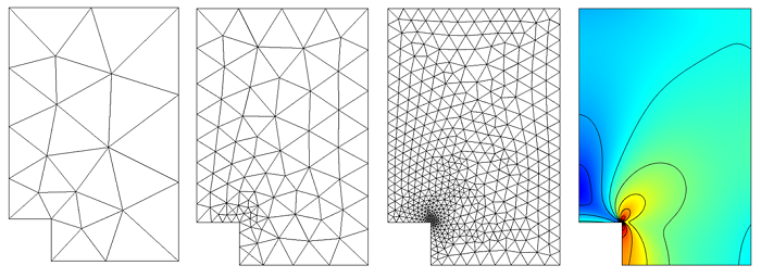
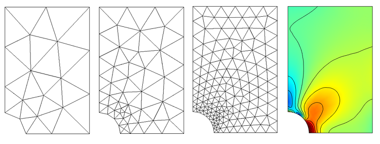
How to Identify and Resolve Singularities in the Model when Meshing
In our previous post on Meshing Considerations for Linear Static Problems, we found that, in the limit of mesh refinement, the solution to the finite element model would converge toward the true solution. We also saw that adaptive mesh refinement could be used to generate a mesh that would have smaller elements in regions where the error was higher, rather than simply using smaller elements everywhere in the model. In this post, we will examine a couple of common pitfalls […]
Meshing Considerations for Linear Static Problems
In this blog entry, we introduce meshing considerations for linear static finite element problems. This is the first in a series of postings on meshing techniques that is meant to provide guidance on how to approach the meshing of your finite element model with confidence.
Solving Linear Static Finite Element Models
In this first blog entry of our new solver series, we describe the algorithm used to solve all linear static finite element problems. This information is presented in the context of a very simple 1D finite element problem, but is applicable for all cases, and is important for understanding more complex nonlinear and multiphysics solution techniques to be discussed in upcoming blog posts.