
By modeling the effects of climate change, scientists can design solutions to mitigate its potential impact. One example is the melting of permafrost in northern boreal regions. Climatologists expect especially large impacts and strong positive feedback loops in these regions. The InterFrost Project designs benchmark cases to test, evaluate, and validate numerical codes and models of subsurface processes. The example here matches an InterFrost benchmark by using a thermal-hydraulic approach to model a melting frozen inclusion in soil of above-zero temperature.
What Is a Frozen Inclusion?
A frozen inclusion is a bit of frozen something inside of a solid something — like the inside of a pizza roll that needs more microwaving. Discontinuous or sporadic permafrost is another example: frozen bits of ice inside of porous (but still a solid) soil. A nonexample is ice cubes in water, as the ice is not encapsulated.
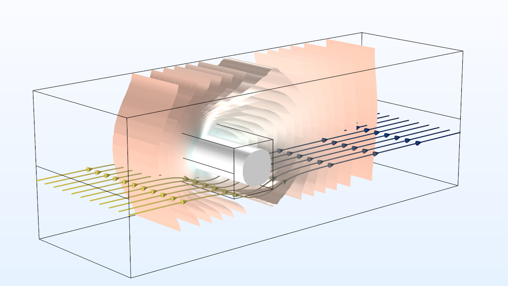
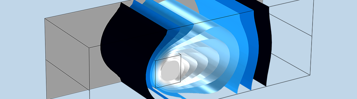
A 3D figure of a frozen inclusion: The results show the ice block within the encompassing channel after 9 h (white surface), the velocity streamlines (colors represent the hydraulic head), and the surrounding temperature (isosurfaces).
Modeling a Frozen Inclusion in COMSOL Multiphysics®
In this example, you can model the phase change of a frozen inclusion from ice into water. How does it melt? How long will it take to melt? How long until all of the cold water is out of the frozen soil?
While this specific benchmark simulation is of particular interest to climatologists and other earth scientists, the concepts shown can also be of use to anyone interested in analyzing phase changes in porous media. For this tutorial, it may be helpful to think about permafrost.
The given geometry is shown below. The channel is 3 meters long and 1 meter wide. The ice inclusion is 33.3 centimeters long, is located at (x,y)=(1, 0.5), and is -5°C. Finally, the hydraulic head gradient is 3% over the length of the channel with a temperature of 5°C. Due to symmetry, only the lower half of the channel is simulated.
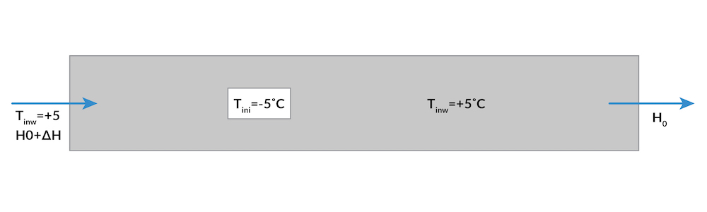
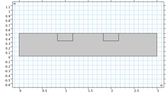
The model geometry, showing the initial temperature distribution and boundary conditions (zero conductive flux, zero flux).
There are certain given numbers, including the temperature of the inclusion, the temperature of the water, the geometry’s size, and the hydraulic head gradient.
There are several equations in this example, most notably Darcy’s Law. You can also assume the following:
- The heat transfer equation has no thermal dispersion
- Water density is constant with temperature
- Water dynamic viscosity is constant with temperature
Examining the Simulation Results
The frozen inclusion melts after only about 20 in-simulation hours. However, it takes a full 56 in-simulation hours for the cooler temperatures to be convected out of the channel (this is because porous media holds temperature better than free media). Take a look at the results…
After 9 hours, the frozen inclusion is still apparent in the soil.

Surface plot showing the temperature distribution after 9 hours.
After 56 hours, the ice is completely melted and the cooler temperatures are almost out of the channel.
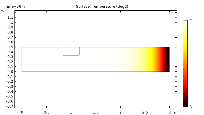
Surface plot showing the temperature distribution after 56 hours.
While this benchmark model is a simple example, it demonstrates that researchers can turn to simulation to analyze similar, yet more complex, problems. For example, what if the frozen inclusion wasn’t rectangular but was sinusoidal instead? Further, simulating problems like these can help climatologists determine when the ice will melt and contribute to water saturation, which leads into a host of geologic questions.
A Second Scenario
To make things more interesting, let’s see what happens if there are two ice blocks in the soil. After all, permafrost has many frozen inclusions by definition. First, another ice block is added in the geometry.
Now, let’s run the simulation again. What do you think will happen?
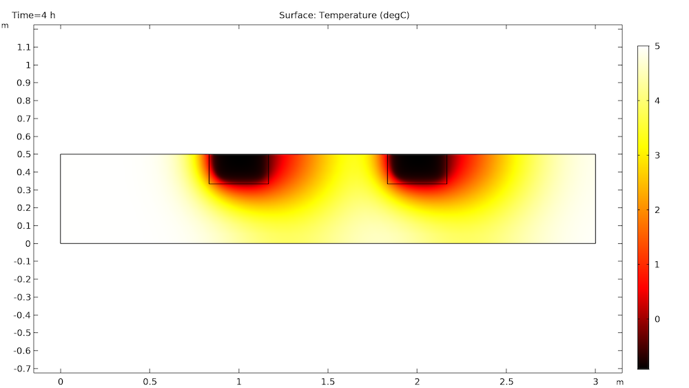
As we can see from the animation above, the ice blocks initially melt at the same rate, but the second ice block’s melt rate slows down after about 9 hours. You can look at the change in temperature gradients to see why.
At first, the blocks melt as individuals in isolation from each other.
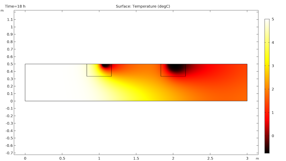
After some time, the cold temperatures from the first block travel downstream to the second block. This decreases the temperature difference surrounding the second block, which in turn decreases the melt rate. This is very clear by 18 hours, as shown below.
The first block melts after 21 hours, but the second block still has a way to go and is still quite affected by the temperature gradient caused by the first block.
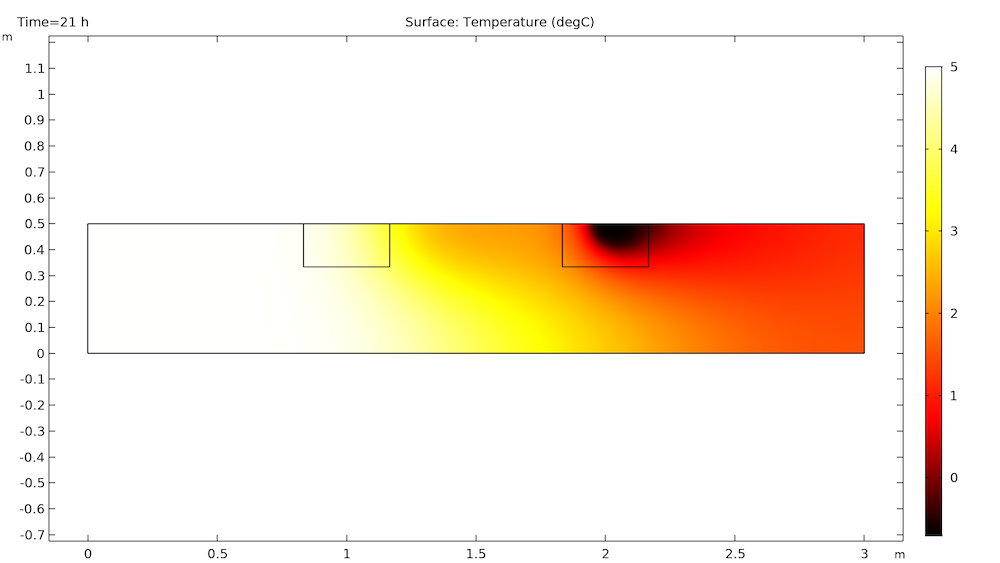
It takes 29 hours for the second block to melt (9 hours after the first block) and 56 hours for the temperature to be convected out of the channel.
Conclusion and Next Steps
The melting of frozen inclusions can be difficult to solve analytically, but simple and more complex problems can be simulated using a thermal-hydraulic approach. As this benchmark, subsequent example, and the InterFrost Project show, simulation is a powerful and accurate tool for modeling melting permafrost and predicting the impact of climate change in northern boreal regions.
This is another example of how COMSOL Multiphysics can be used to create models and simulations regarding environmental problems. Other examples include:
Try modeling the melting of frozen inclusions yourself with the Frozen Inclusion tutorial model by clicking the button below. Doing so will take you to the Application Gallery, where you can download additional PDF documentation and an MPH file.

Comments (0)