
High-intensity focused ultrasound (HIFU) is a noninvasive procedure used for biomedical applications including surgery, cancer therapy, and shock wave lithotripsy. When HIFU is applied, ultrasonic waves are dissipated at a focal point for tissue coagulation and ablation. The acoustic characterization and nonlinear nature of this technique can be further analyzed with the help of simulation.
Ultrasound Focusing for Medical Procedures
For procedures used in clinical applications, ultrasound focusing is a widely used technique that targets specific areas of the body and prevents the risk of damage to surrounding healthy tissue. HIFU is similar to ultrasonic imaging, but it is a less invasive technology that uses lower frequencies, reducing side effects typically seen with other treatments.
HIFU uses an ultrasound transducer with a focusing lens, where the emitted signal can reach higher intensity levels within a focal zone. Nonlinear effects become significant and generate higher-order harmonics when the signal reaches a high amplitude. Using the COMSOL Multiphysics® software and the Acoustics Module, we can model the nonlinear propagation of HIFU through a dissipative media.
Modeling an Ultrasonic Signal Within a Focal Zone
The transducer housing and lens used in this tutorial model are assumed to be rigid. The spherical lens of radius (r) and aperture (a) emits a five-cycle tone burst pulse that is focused at the focal point F located in the tissue phantom. The signal, which will only occupy a limited part of the domain as it travels, has an amplitude of 0.1 MPa and a center frequency of 1 MHz. The amplitude is significant enough to generate higher-order harmonics while the signal is propagating, but it is not high enough for the formation of shocks, meaning no shock-capturing techniques are required.
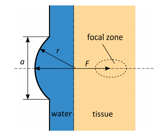
Illustration of the 2D axisymmetric model geometry.
We can calculate the traveling time from the signal to the focal point with:
where c is the speed of sound and d is the traveling distance in the corresponding materials.
Using the Nonlinear Pressure Acoustics, Time Explicit interface, available as of COMSOL Multiphysics version 5.6, we can model finite-amplitude high sound-pressure-level nonlinear waves in fluids. For this tutorial, the interface solves the system of nonlinear acoustic equations in the form of a hyperbolic conservation law, using the discontinuous Galerkin finite element method (dG-FEM). This is a more memory-efficient approach that can solve models that have many million degrees of freedom (DOFs).
Typically, when solving a wave propagation problem, the mesh would need to be fine enough to resolve the frequency content of the signal. The model used in this tutorial features the source as a pulse, making the propagating signal finite in space. In this case, a fine mesh is only required in this part of the computational domain (saving many DOFs). To implement this, adaptive mesh refinement is enabled for automatic remeshing, which ensures a fine-enough mesh for resolving the propagating signal’s higher-order harmonics.
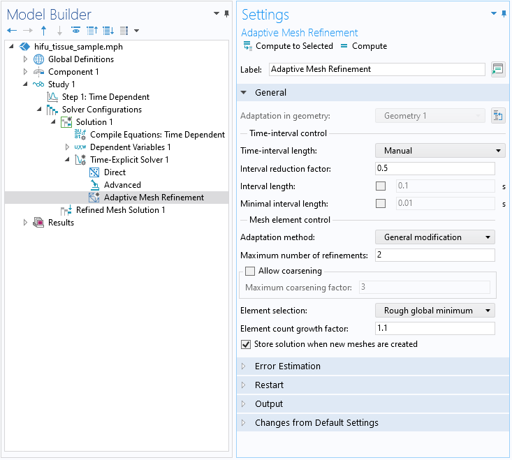
Settings for the Adaptive Mesh Refinement feature.
Analyzing the Propagation of the HIFU Signal
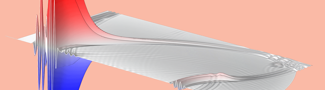
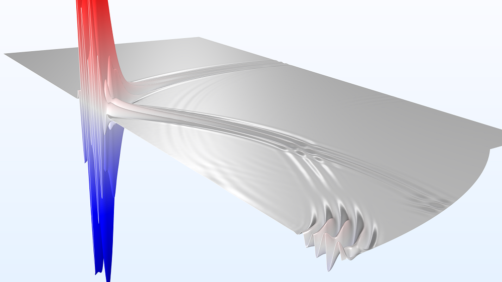
From the results below, we can see the tone burst signal starts at t = 10 μs and proceeds to travel between the water and tissue phantom domains. We are also able to visualize part of the signal being reflected back to the source at t = 20 μs. Additionally, the focusing of the signal becomes visible at t = 30 μs and reaches its maximum at t = 40 μs. These results show that as the signal becomes closer to the focal zone, the signal strength increases.


Propagation of the ultrasonic signal at times t = 10, 20, 30, and 40 μs.
We can confirm the results above by analyzing the signal at the water–tissue interface and focal point. From the plot below, we are able to see that at the focal point, the acoustic pressure amplitude is about 10 times greater than at the water–tissue interface. Also, at the focal point, the positive pressure peaks are almost twice as high as the negative peaks, an indication that the signal becomes highly nonlinear as it travels toward the focal zone.
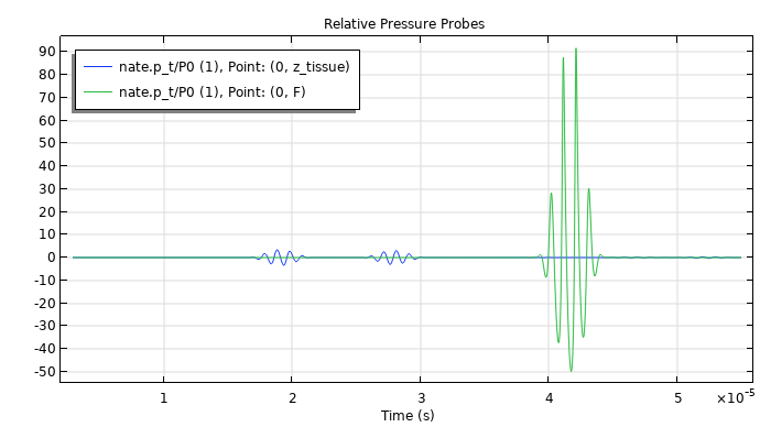
Acoustic pressure at the water–tissue interface and focal point.
As mentioned earlier, the Adaptive Mesh Refinement feature was used for automatic remeshing while following the signal through the computational domain. The animation below shows how the mesh follows the nonlinear propagation of the signal. The mesh in this case has smaller elements around the sharp fronts and the larger elements are located further away.
Next Step
Click the button below to try out the model for yourself. This will take you to the Application Gallery, which includes step-by-step documentation and an MPH file.


Comments (0)