
Due to the complex pumping scheme of high-power CO2 lasers, there are many species and collisions to consider in their analysis. This makes modeling plasma behavior in these devices — a key element in their optimization — a challenging task. Applying a multilevel approach, one researcher used the COMSOL Multiphysics® software to create a full 3D model of planar discharge in a CO2 laser. The results showcase the homogeneity of the discharge while offering further potential for optimizing laser designs.
The Importance of Plasma Behavior in CO2 Lasers
When CO2 lasers first arrived on the scene in 1964, they represented one of the earliest of their kind — a gas laser. Since then, these high-power devices have been used extensively in materials processing applications, such as sheet metal cutting and welding.
With continued advancements in these fields and the goal of extending into new applications, improving the power and stability of CO2 lasers has become a point of emphasis. One element that is key to such optimization is the modeling of plasma behavior inside the laser. These analyses are useful in improving (among other things) the gas dynamics within the laser; the cooling design; and, as we’ll highlight in more detail here, the homogeneity of the discharge.
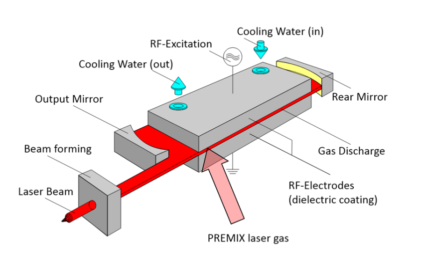
Consider the diffusion-cooled slab laser design below. In this configuration, the plasma forms between two planar electrodes that serve as an optical waveguide and also cool the gas.
The diffusion-cooled slab laser design. Image by J. Schüttler and taken from his COMSOL Conference 2016 Munich paper.
Like other CO2 lasers, the design includes a complex pumping scheme. Because of this, there are a large number of species and collisions to take into account. From a modeling perspective, this creates a complex multiphysics problem that is difficult to solve within a practical amount of time.
To make this problem more manageable to solve, a researcher from Rofin-Sinar Laser GmbH in Germany used a multilevel approach to create a full 3D model of planar discharge in the CO2 laser. While the model itself is quite advanced, it is a great example of what is possible with the flexibility and functionality available in COMSOL Multiphysics.
Modeling of Planar Discharge with a Multilevel Approach
1. Analyzing the Steady-State Behavior of Plasma
The laser configuration shown above includes a premixed gas comprised of six components, which together are designed to provide efficient cooling and long-term stability. The table below provides an overview of each component.
| Gas | Volume | Function |
|---|---|---|
| He | 65% | Cooling |
| Xe | 3% | Preionization |
| O2 | 3% | Electron attachment |
| N2 | 19% | Resonance energy transfer to CO2 |
| CO2 | 4% | Lasing transition |
| CO | 6% | Long-term stability |
Because of the large number of species involved, the electron energy distribution function (EEDF) is not known a priori. To calculate the EEDF, as well as the reduced transport properties and reaction rate coefficients for the premixed gas, the researcher used the Boltzmann Equation, Two-Term Approximation interface.
In the plot below, we can see the attachment and ionization rates for varying reduced electric fields. These results are used as interpolation functions for subsequent simulation steps.
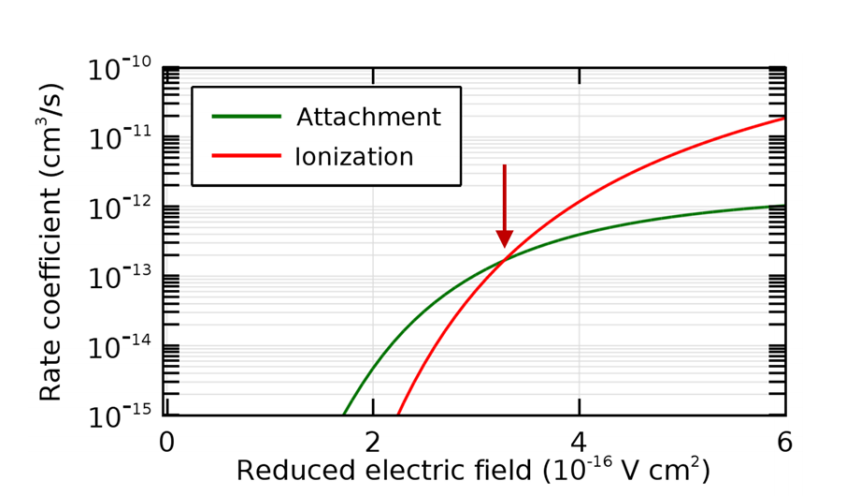
Rate coefficients for attachment (green) and ionization (red) for varying reduced electric fields. The red arrow indicates the value of the reduced electric field where attachment and ionization balance. Image by J. Schüttler and taken from his COMSOL Conference 2016 Munich paper.
2. Examining Gas Discharge Properties in the Electrode Gap
To simulate the discharge, the researcher used the Plasma interface. The figure below depicts the geometry of the 1D model as well as its boundary conditions. The 1D domain is bound by the electrode surfaces (a and g) with a dielectric material coating (b and f). The interval d represents the point at which the plasma model, reactions, and species are defined.
For details on how to model a dielectric barrier discharge, see this example in the Application Gallery.
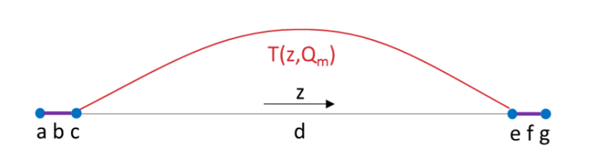
1D discharge geometry. Image by J. Schüttler and taken from his COMSOL Conference 2016 Munich paper.
Note that in order to accurately describe the discharge behavior, the gas temperature must be self-consistent according to the heat that is dissipated during discharge. Because the maximum temperature depends solely on the average heat source within the gap, an artificial time scale, T(z, Qm), is used. This ensures fast convergence of the gas temperature to the quasi steady state solution.
An example of the spatiotemporal evolution of the electron density in the discharge gap is shown below. Following a few RF cycles, the discharge begins and the electron density rapidly increases from low preionization to a more significant level. After some time, the electron density and temperature reach a nearly stationary state.
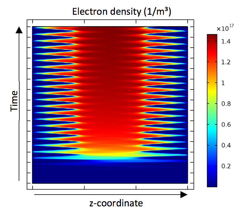
The spatiotemporal evolution of electron density within the discharge gap. Image by J. Schüttler and taken from his COMSOL Conference 2016 Munich paper.
Important results are also obtained for various discharge characteristics, including terminal voltage. Note the area labeled NDR, which stands for negative differential resistance. This thermal effect, caused by the nonlinear behavior of the ignition of plasma past a threshold voltage, is an important feature of the discharge — one that can only be observed in self-consistent calculations of temperature. The solution in this region is bistable for a prescribed terminal voltage. Once again, this information can be used as an input in the 3D simulations.
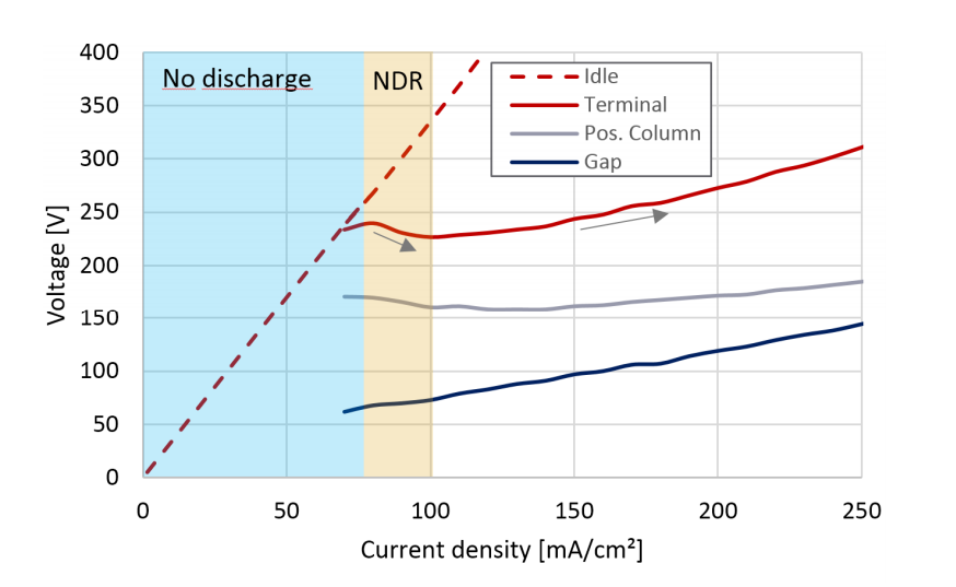
The voltages over an applied terminal current density. Image by J. Schüttler and taken from his COMSOL Conference 2016 Munich paper.
3. Using Response Curves in Large-Scale RF Simulations
Reproducing this behavior within the large-scale RF simulations called for the design of a surrogate material. This material replaces the plasma discharge with a strongly nonlinear conductive sheet of material, placed between the electrodes. Note that on each side, the sheet is separated from the electrodes by a distance (ds).
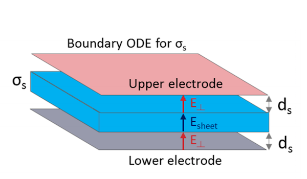
The setup for the surrogate material. Image by J. Schüttler and taken from his COMSOL Conference 2016 Munich paper.
When computing the electric potential along the discharge gap for two solutions in the bistable region, both solutions — with ignited plasma (blue) and without ignited plasma (red) — have the same potential at the terminal boundary conditions. However, their electric fields differ. These unique solutions can be found via the electric field at either electrode surface.
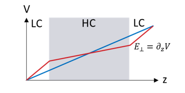
Ambiguous solutions for terminal voltage. Image by J. Schüttler and taken from his COMSOL Conference 2016 Munich paper.
Through a parametric study performed with the Electric Currents interface, the minimum phase angle between the voltage and current at the terminal boundary condition is shown to depend solely on the gap distance. An interpolation function set up at a later point indicates the same dependency as that described in the plasma simulations.
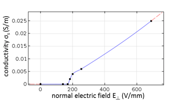
Interpolation function used as a surrogate material. Image by J. Schüttler and taken from his COMSOL Conference 2016 Munich paper.
Solving the macroscopic RF simulations in 3D requires the use of the Electromagnetic Waves interface and a frequency-domain solver. The domain consists of the gas volume enclosed within the structure and a few domains comprised of dielectric materials. RF power is applied to the calculation domain at several coaxial ports located near one of the long sides of the electrodes. The mesh is comprised of 913,564 elements, which results in 6,737,446 degrees of freedom.
Evaluating Simulation Results for the CO2 Design
Now that we’ve reviewed the approach, let’s take a look at the obtained results.
In the example below, we can see the current density distribution of the gas discharge. The discharge is found to be homogeneous within a range of around 10%. When compared to experimental observations for various parameter regimes and configurations, the results from the simulation show good agreement.
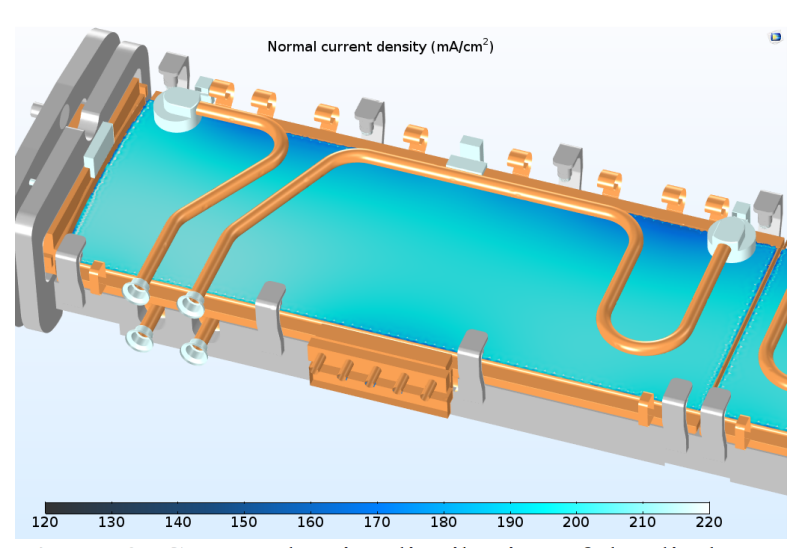
The current density distribution of the discharge. Image by J. Schüttler and taken from his COMSOL Conference 2016 Munich paper.
Verification of this modeling approach has encouraged its use in subsequent development tasks, including the design of a new RF feed and the prediction of stable working points for other types of gas compositions. As for this specific model, there are future plans to further extend it to address the temporal evolution of the ignition phase. This would not only enable the analysis of pressure variations when the laser is switched on, but it could also improve the laser’s performance in pulsed operation.
Resources on Modeling High-Power Laser Systems with COMSOL Multiphysics®
- Read the full COMSOL Conference paper: “3D Modeling of Planar Discharge of a CO2 Laser“
- Browse additional blog posts relating to the optimization of high-power laser systems:
Comments (0)