

Transmission lines are used to propagate energy for the communication of a signal from input to output ports. Examples include waveguides, coaxial lines, planar transmission lines, microstrip lines, coplanar waveguide lines, and slot lines. For the successful deployment of microwave systems, engineers use various types of transmission lines where the electromagnetic wave is coupled from one type of transmission line into another through appropriate transitions. These transitions should have low transmission and reflection losses.
Main Transition Types for Rectangular Waveguides
The different types of transitions that are frequently used in microwave circuit design are discussed in this blog post as follows:
- Waveguide to planar transition
- Coaxial to waveguide transition
- Rectangular to elliptical waveguide transition
1. Waveguide to Planar Transmission Line Transition
Waveguides are a suitable candidate for handling high-power and low-loss transmission, but they are also bulky and expensive. Planar transmission lines, such as microstrip lines, have gained popularity in the microwave field because of their compact size and ease of integration with transistors and diodes to form microwave-integrated circuits (MICs). For these reasons, a transition between a waveguide to a planar transmission line is suitable for many types of microwave systems.
Waveguide to planar transmission line transitions can be broadly classified into three types:
- In-line transition: Transition takes place along the propagation of the waveguide
- Aperture coupling transition: Energy is coupled to the planar transmission line via the aperture, which can be present at the endwall or broadwall of the waveguide
- Transverse transition: The probe is transverse to the propagation direction of the waveguide
Considering the third type of transition, the waveguide to microstrip line transition model is discussed in detail. In this model, a standard WR10 waveguide is used, and transition from the waveguide to the microstrip line is achieved by using the longitudinal probe (also known as the E-plane probe) transverse to the propagation direction of the wave. The longitudinal probe is inserted from broader sidewalls of the waveguide, where the surface of the substrate aligns along the direction of propagation of the waveguide (Ref. 1).
Back-to-back transition of the waveguide to microstrip line transition model.
In this model, the microstrip line is designed along with a quarter-wave transformer to match the impedance to 50 [ohm] on a RT/duroid® 6010LM laminate substrate, which is available in the RF Module material library of the COMSOL Multiphysics® software.
To easily set up the model experimentally, the design is extended to back-to-back transition. In this extended design, a 50 [ohm] microstrip line is converted back to the probe, which acts as a feeder for an adjacent WR10 waveguide. To account for losses at a higher frequency, appropriate boundary conditions are used. For example, the Impedance boundary condition (IBC) is used for the waveguide walls (suitable when the thickness of the conductor is larger than the skin depth) and the Transition boundary condition (TBC) is used for microstrip lines (suitable when the conductor thickness is comparable with the skin depth), which helps to make the numerical model close to an experimental setup. Another approach involves the use of a perfect electric conductor (PEC); however, the PEC is a lossless condition and hence is not used in this model.
It can be observed from the S-parameter plot that the reflection is below -15 dB in the entire band (75 GHz to 110 GHz), while maximum transmission loss is observed as 0.7 dB. A Smith plot for S11 revolves very closely around the center, which implies good matching. This kind of transition setup is relevant for the automotive industry, where radar technology is now shifting from the K-band to W-band because of several advantages, such as huge bandwidth, high resolution, and reduction in antenna size.


S-parameter response and Smith chart of S11 for the waveguide to microstrip line transition model.
2. Coaxial to Waveguide Transition
The second transmission line transition we discuss in this blog post is a coaxial to waveguide transition. The coaxial line can be used as a feeder for the waveguide, as shown in the coaxial to waveguide model.
This model demonstrates a simple coaxial to waveguide transition using the RF Module and COMSOL Multiphysics. The incoming wave through the coaxial cable is set up using a Port boundary condition with a 1-W coaxial feed. At the passive output port, the fundamental rectangular TE10 mode is assumed. The Port boundary conditions are perfectly transparent only to their specified mode. These same modes are also used for quantifying the S-parameters automatically.
For such reasons, the modeled sections must be long enough so that the evanescent waves almost completely die out before they reach the ports. This leaves us only with the propagating modes at 6 GHz, the only supported propagating mode (i.e., the fundamental mode). In this case, to account for the losses, the Impedance boundary condition with the material property for copper is used for the coaxial conductors and metal surfaces of the waveguide.
Coaxial to waveguide coupling with E-field distribution.
3. Rectangular to Elliptical Waveguide Transition
An elliptical waveguide can be deployed in microwave backhaul due to its optimal performance and minimum field errors. Bending or flaring devices are typically formed by converting a traditional rectangular waveguide into an elliptical waveguide. Such devices are designed in such a way that energy losses due to reflections are minimum for the operating frequencies.
For example, in the Waveguide Adapter model, microwave propagation in the transition between a rectangular waveguide and an elliptical waveguide is analyzed. To investigate the characteristics of the adapter, this example includes a wave traveling from a rectangular waveguide through the adapter and into an elliptical waveguide. The S-parameters are calculated as functions of the frequency. The involved frequencies are all in the single-mode range of the waveguide; that is, the frequency range where only one mode is propagating in the waveguide.
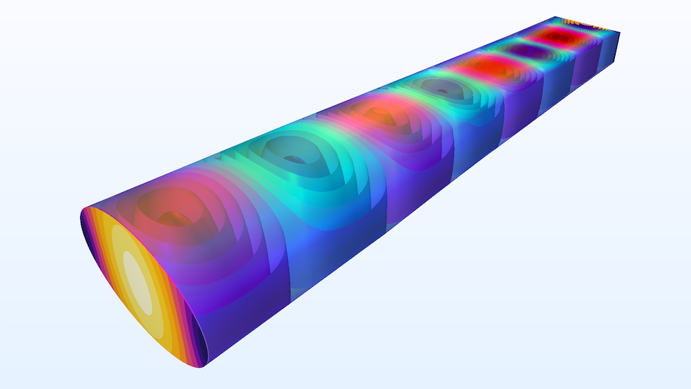
Isosurface plot of the x-component of the electric field in a rectangular to elliptical waveguide transition.
Concluding Thoughts
Transmission line transitions are frequently used and should have low reflection losses and low transmission losses. At higher frequencies and due to the finite conductivity of metal used in the transmission line, the skin effect, which is responsible for the transmission loss, becomes predominant. To account for this loss, boundary conditions such as IBC and TBC can be used appropriately, with minimum computational cost, while reflection losses can be minimized by impedance matching.
Next Steps
Try modeling a transmission line transition in COMSOL Multiphysics by checking out the three tutorial models discussed in this blog post:
Reference
- Yoke-Choy Leong and S. Weinreb, “Full band waveguide-to-microstrip probe transitions,” 1999 IEEE MTT-S International Microwave Symposium Digest, pp. 1435–1438 vol. 4, 1999.
RT/duroid® is a registered trademark of Rogers corporation or one of its subsidiaries.

Comments (0)