Polymer Flow Module
COMSOL Multiphysics® version 5.6 introduces the new Polymer Flow Module. This product is an add-on to COMSOL Multiphysics® and contains viscoelastic and inelastic non-Newtonian models for describing fluids that are found in a variety of processes in the polymer, food, pharmaceutical, cosmetics, household, and fine chemicals industries. The Polymer Flow Module also features methods for free surface tracking in order to predict the shape of the liquid–air interface in the application of coatings, mixing of liquids, and in the filling of molds.
Viscoelastic Fluid Models
Viscoelastic fluid models account for the elasticity in these types of fluids. As the fluid is deformed, there is a certain amount of force that works toward returning the fluid to its undeformed state. Typical examples of these fluids are polymer melts, paints, and suspensions of proteins. The Polymer Flow Module features a variety of viscoelastic fluid models such as the Oldroyd-B, Gisekus, FENE-P, and LPTT models. The models can predict the forces exerted by the fluid, the uniformity of coatings as they are applied, and the degree of mold filling in processes involving the curing of polymers.
Inelastic Non-Newtonian Flow Models
In addition to the viscoelastic fluid models, the Polymer Flow Module features a wide range of inelastic non-Newtonian models. Many of the models are generic, used to describe shear thinning and shear thickening. For more specific applications, there are models for viscoplastic and thixotropic fluids. Colloidal suspensions may exhibit shear thickening behavior, where viscosity increases substantially with shear rate. Other suspensions may be shear thinning, for example syrups and ketchup, where the viscosity decreases with shear rate. Thixotropic fluids also have a time dependency, where the viscosity decreases with the duration of the shear rate. The models describing these fluids are all inelastic but they describe highly non-Newtonian behavior.
Multiphase Flow Models
To model the liquid–air interface when simulating coatings, free surfaces, and mold filling, the Polymer Flow Module includes three different separated multiphase flow models based on surface tracking methods: The Level Set, Phase Field, and the Moving Mesh methods.
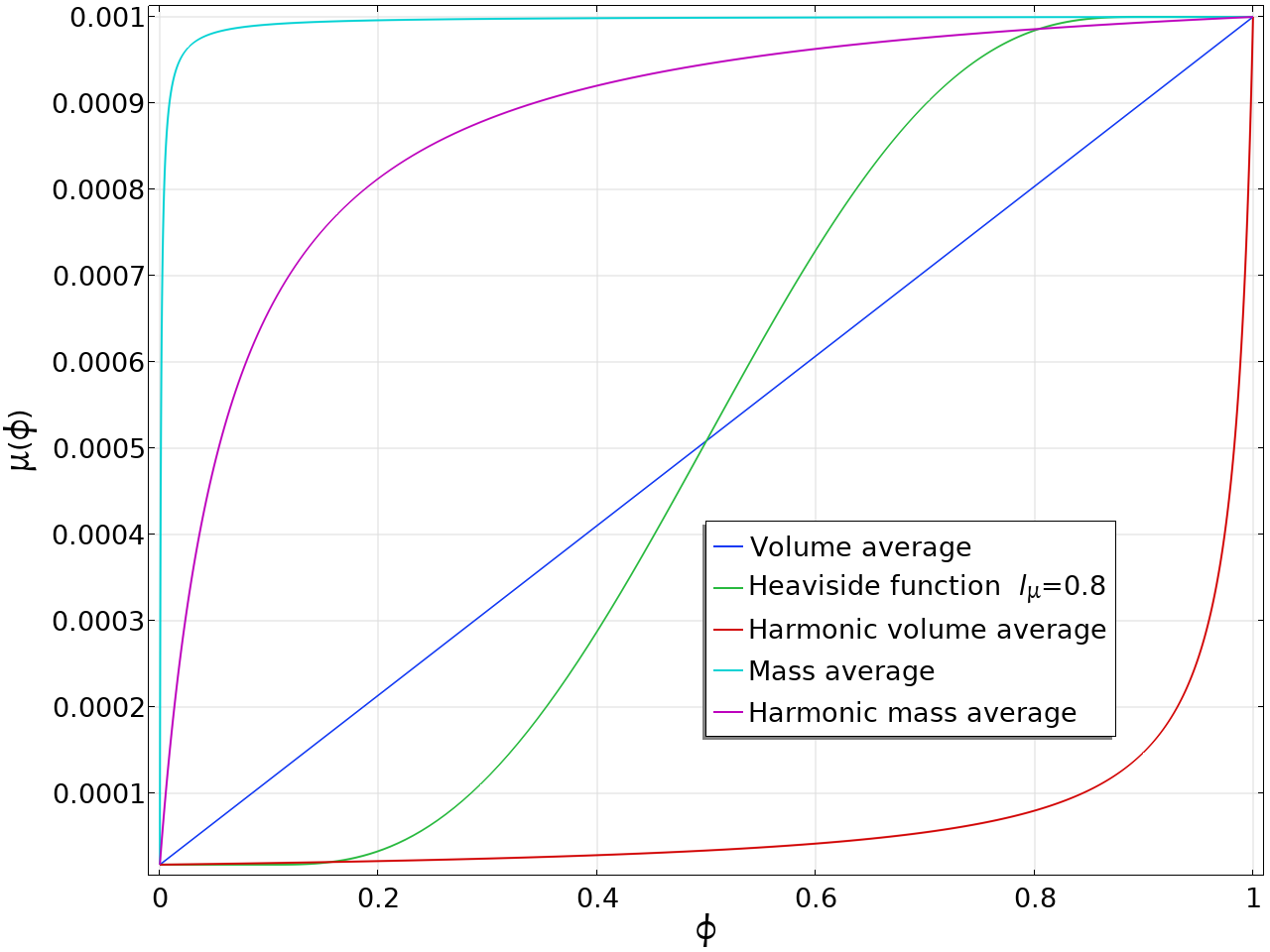
New Averaging Options for Fluid Properties Across Phase Interfaces
When the density and/or viscosity ratio in a two-phase flow simulation is large, the use of volume-averaged fluid properties across the phase interface may lead to excessive smearing. Sharpening the transition zone for the fluid properties, or displacing it into one of the two phases, may improve accuracy and/or convergence in some cases. In version 5.6, smoothed Heaviside functions and harmonic volume averages can be used for both density and viscosity. For the viscosity, mass averaging and harmonic mass averaging are also available as options.
Easier Setup for Phase Field and Level Set Models
The Level Set and Phase Field interfaces have been restructured: Two Initial Values nodes are now added by default, and the previously used Initial Interface feature has been removed. Instead, the initial interface is automatically placed at the boundaries between the two Initial Values nodes with different initial phases.
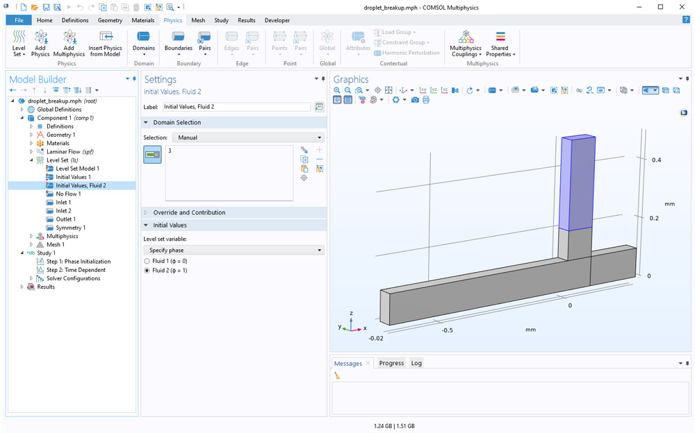
Settings for the Initial Values, Fluid 2 feature. Note that the Initial Interface feature is no longer needed. The initial distribution of the level set or phase field function is solved for in the Phase Initialization study step.
New Tutorial Models
The Polymer Flow Module comes with several tutorial models.
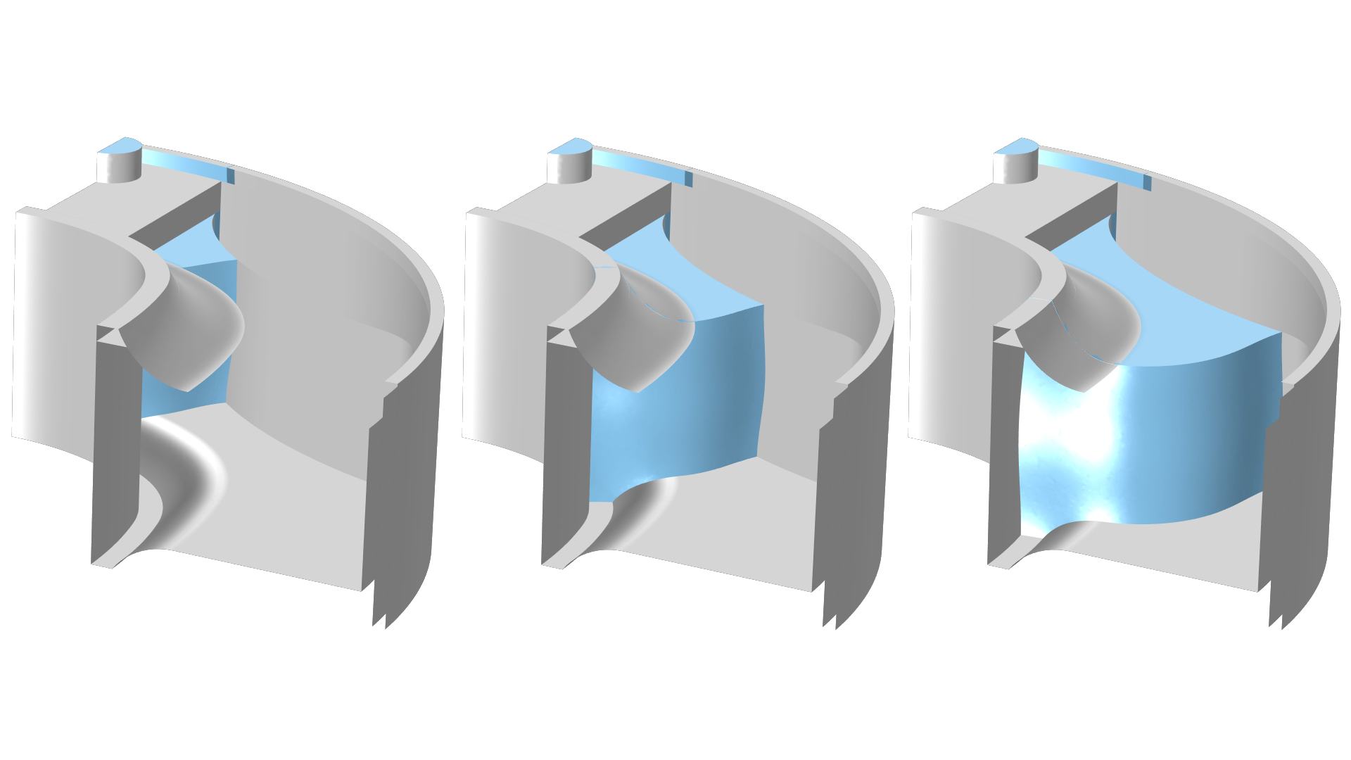
Rubber Injection Molding

Application Library Title:
rubber_injection_molding
Slot Die Coating 2D
Application Library Title:
slot_die_coating_2d
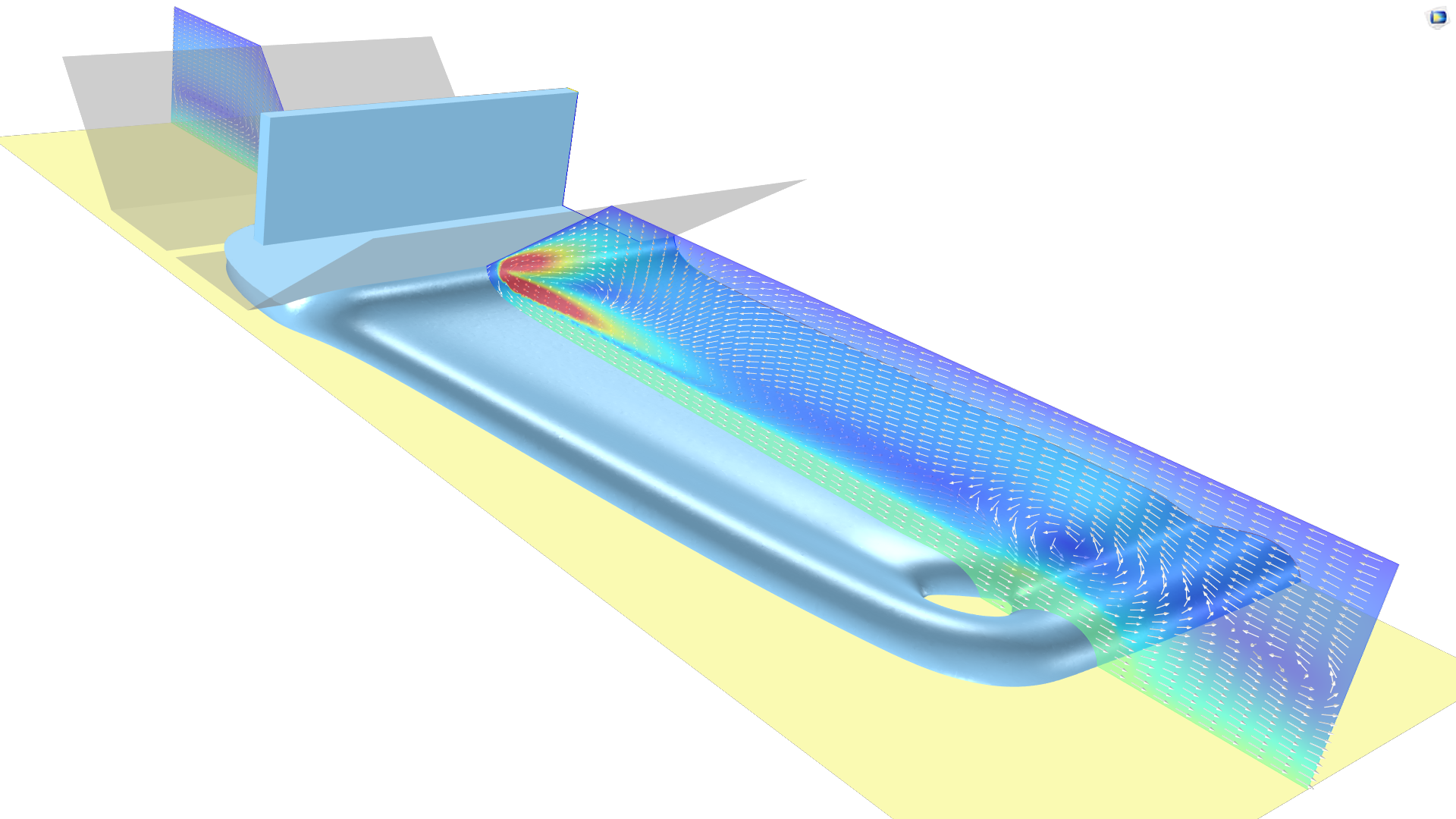
Slot Die Coating 3D
Application Library Title:
slot_die_coating_3D
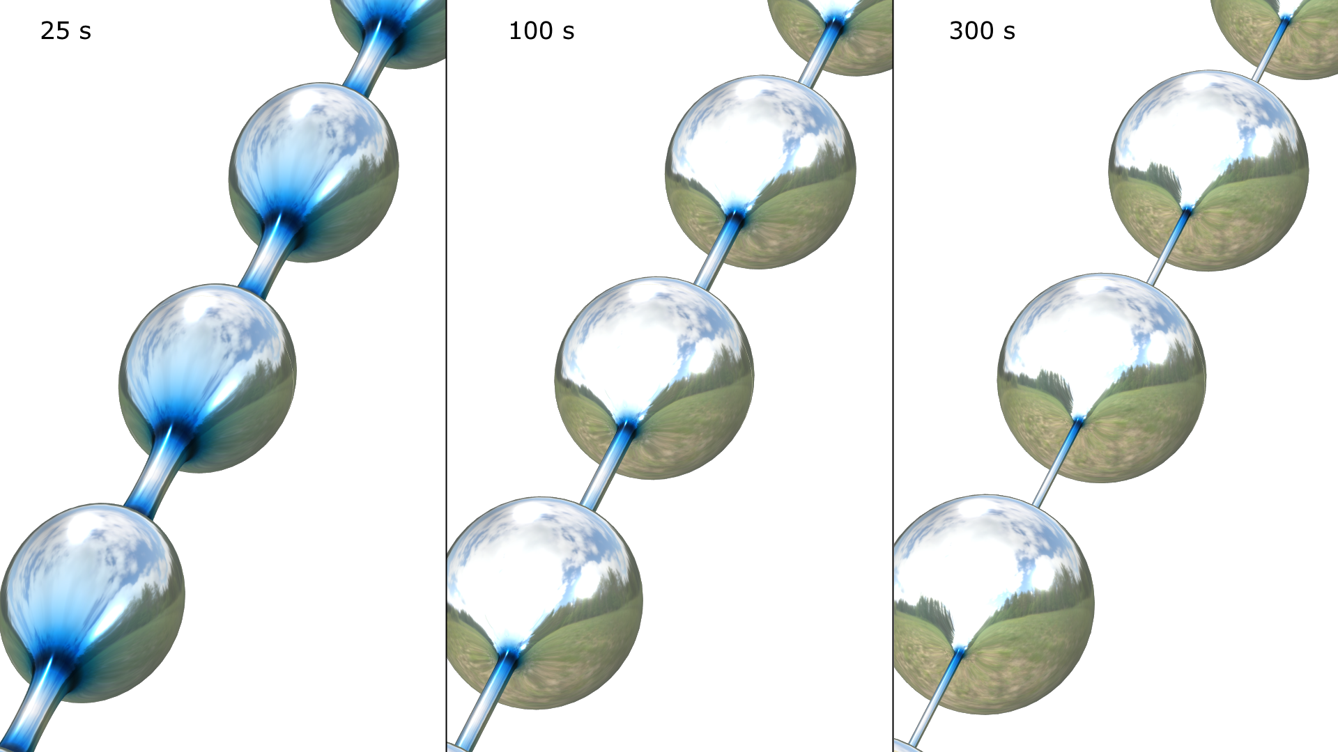
Beads on a String
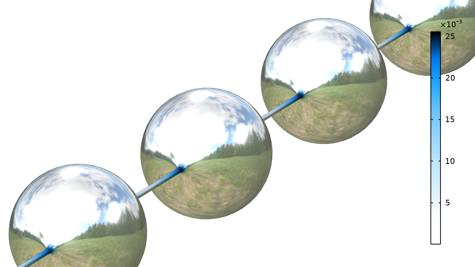
Application Library Title:
beads_on_a_string
Cylinder Flow, Viscoelastic
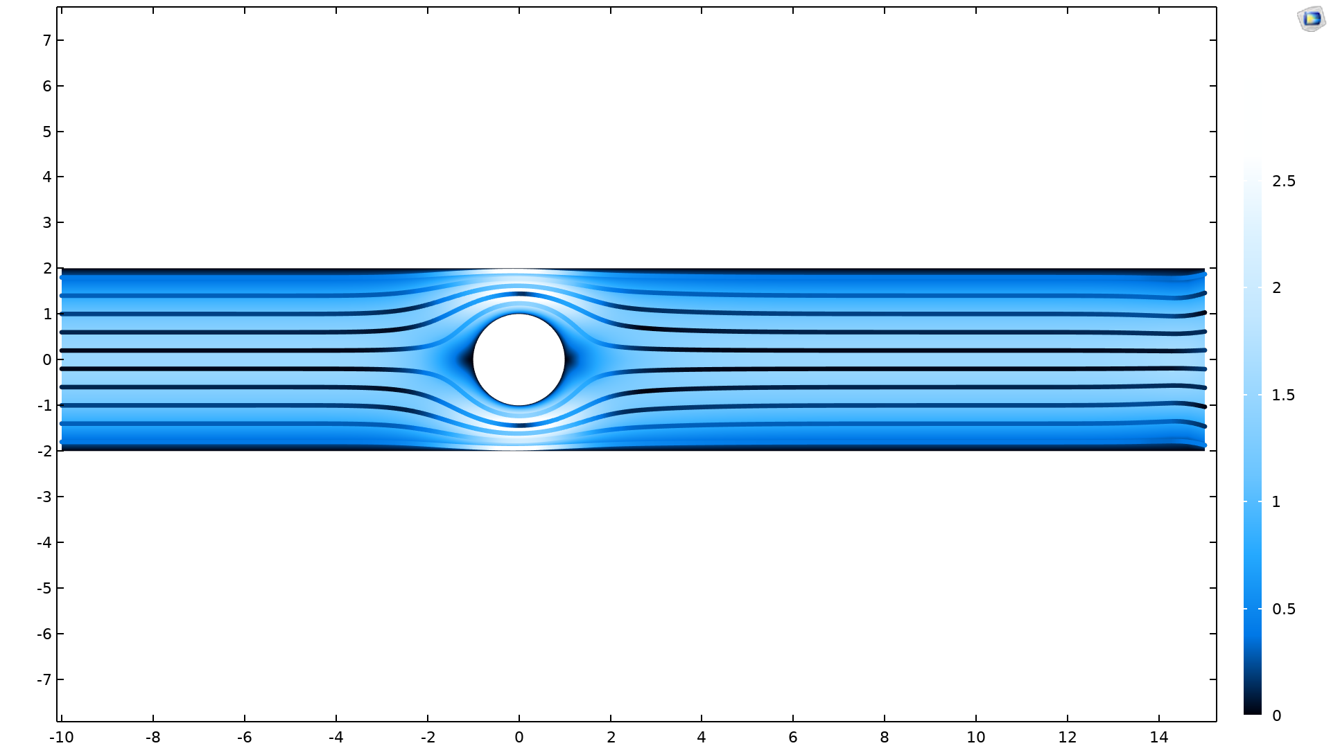
Application Library Title:
cylinder_flow_viscoelastic
Power Law Mixer
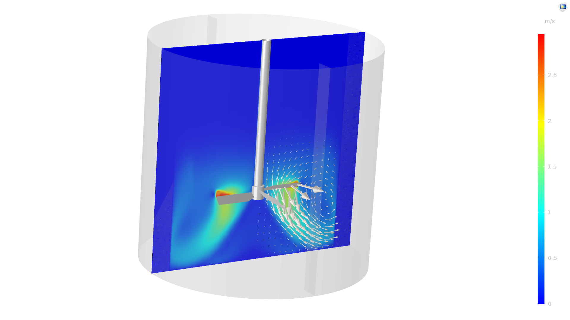
Application Library Title:
power_law_mixer
Carbopol is a registered trademark of Lubrizol Advanced Materials, Inc.