
One of the more common questions we get is: What is the best way to evaluate stresses in the presence of singularities? The most accurate answer is to avoid doing so. However, that is of little help for practical engineering. In this blog post, we take an in-depth look at the properties of singular stress fields and discuss some possible approaches.
This is a follow-up to our blog post “Singularities in Finite Element Models: Dealing with Red Spots”, which describes when and why singular stresses appear in structural mechanics models. It offers a general introduction to singularities and is the recommended starting point if you are new to this topic. For detailed information on how to handle singular stress fields, keep reading here.
A Closer Look At Singular Stress Fields
Let’s start by looking at a more detailed analysis of singular stress fields and their relation to stress concentrations. There are similarities in that a stress concentration also appears at a geometrical discontinuity. The difference between a stress concentration and a singularity is that in the case of the former, the maximum stress is bounded. You can, for example, obtain an accurate value by using a fine-enough mesh in a finite element (FE) model.
Usually, mechanical designers try to reduce the stress concentration by introducing a fillet with as large of a radius as possible. The peak stress at a stress concentration is usually described as the product of a stress concentration factor K_{\mathrm t} and a suitably selected nominal stress. For a fillet, the following expression can sometimes be used for K_{\mathrm t}:
Here, \rho is the fillet radius and L_\mathrm{char} is a characteristic length of the notch that ends in the fillet.
The background to the equation is the analytical solution for the stress concentration at an elliptical hole in a large plate, where L_\mathrm{char} is the length of the larger semiaxis of the ellipse.
A large plate with an elliptical hole.
For most notches, this expression can only be used to provide crude estimates to K_{\mathrm t}, since it’s difficult to deduce the characteristic length. The importance lies in the fact that the peak stress at a small notch will vary essentially as the inverse of the square root of the fillet radius. Any engineer who has tried to reduce a local stress concentration has probably struggled with this fact, since a moderate increase of the fillet radius gives an even more moderate reduction of the peak stress.
The ultimate stress concentration occurs at a crack tip, where the notch radius is infinitely small. In an elastic solid, the solutions for the stress and strain fields close to the crack tip are well known. They vary inversely with the square root of the distance from the crack tip, r. The stress field is commonly written as
Here, K_I, K_{II}, and K_{III} are the stress intensity factors for mode I (opening), mode II (shearing), and mode III (tearing), respectively. The functions f, g, and h consist of trigonometric functions of the polar angle around the crack tip, \theta. (Detailed definitions can be found here.)
An amazing conclusion is that the stress field around a crack tip looks the same, independent of the actual shape of the crack as well as the component in which it exists, as long as you are close enough to the crack tip.
Under the assumptions of linear elastic fracture mechanics, the criterion for fracture in mode I is K_I = K_{Ic}, where K_{Ic} is a material parameter (called fracture toughness). In this way, it’s possible to study geometries with this special type of singularity without explicitly using the infinite stresses. This idea will be generalized in the following text.
Now consider a case where the geometry has something that is almost a singularity. That is, a corner or a crack with a small fillet radius. This is the scenario we will focus on in this blog post. At a distance, we cannot really tell the difference between a notch and a singularity. The following example will elucidate the meaning of this statement.
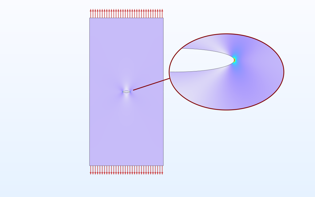
A 2D model of a long notched strip in tension is used. By adding symmetry conditions along the left vertical edge, the same model can also be used for investigating an internal slit.
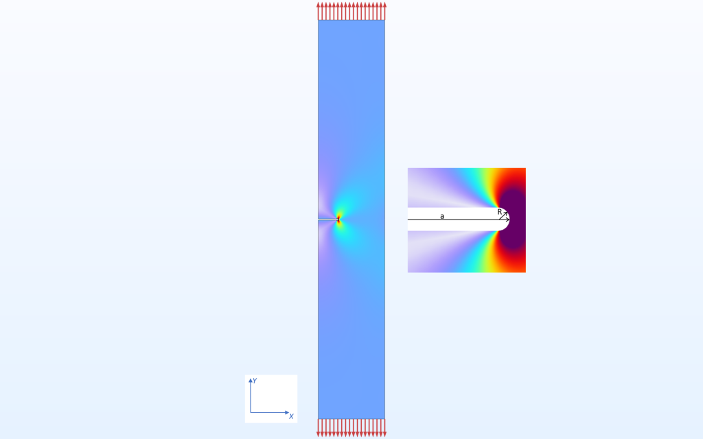
Stress distribution in the notched strip. The model is parameterized with respect to the notch depth
(a) and the notch radius (R).
First, we can note that for a sharp crack, the stress intensity factor for this geometry can be written as
Here, a is the crack length; \sigma is the applied stress (in this case, 1 Pa); and W is the width of the strip. There are several representations of the function f. Here, we will use the expression
This expression gives what is called the crack solution in this blog post.
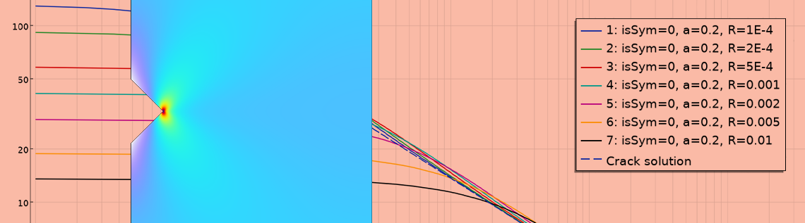
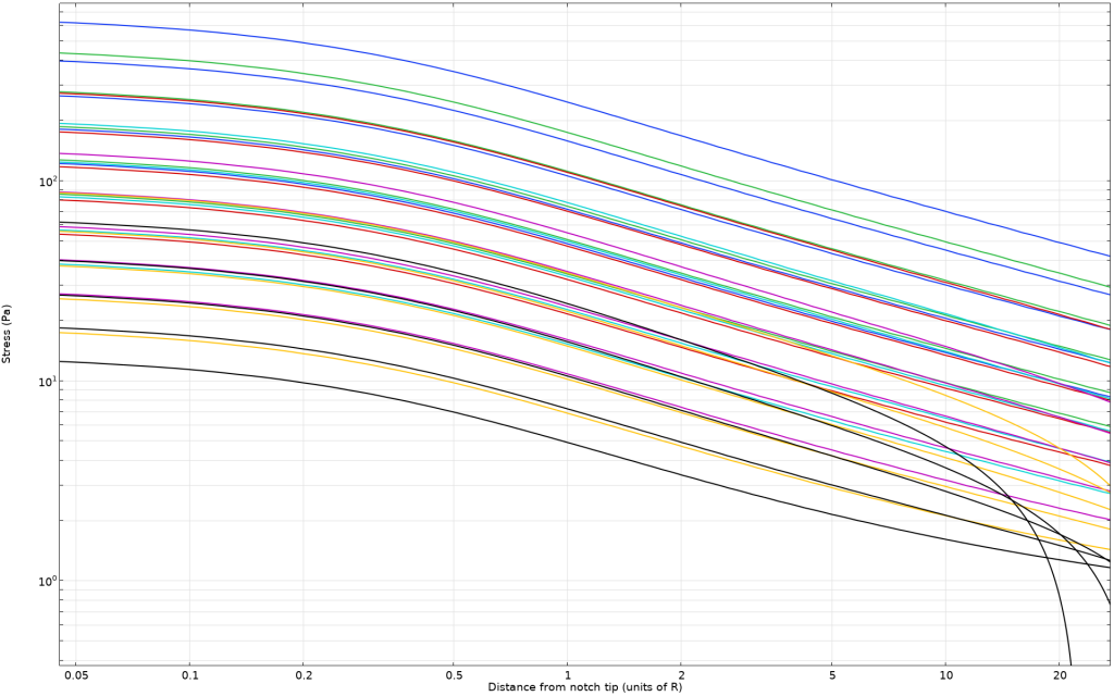
The stress distribution along the ligament (extending in the x direction from the notch tip) is plotted for a short notch and several different notch radii. Due to the symmetry, only one stress component, c, is nonzero.
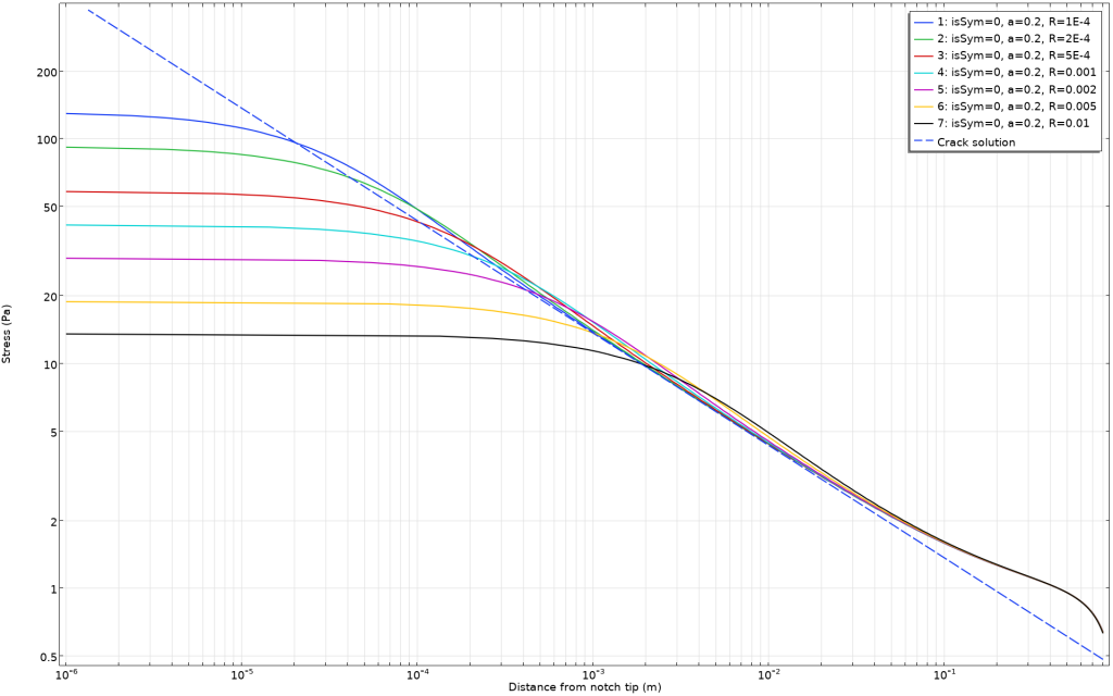
Vertical stress along the ligament as a function of distance from the notch tip for different notch radii. The dashed line shows the theoretical value for a crack with the same depth.
An interesting observation is that in a certain regime, the stress field closely resembles the one obtained for the crack solution. That is, the straight line in the log(stress)-versus-log(distance) diagram. Closer to the notch, the stress is bounded since it’s a notch, not a crack. As expected, the peak stress is proportional to 1/\sqrt{R}.
Far from the tip, the local stress field solution for a crack is not valid anyway, irrespective of whether it’s a crack or a notch. But in the region between very close and far away, both from our visual perspective and from the perspective of the physics and mathematics, it’s not really possible to deduce the true shape of the notch tip.
So why is this important? If we know the shape of the notch, we can actually determine the stress there, just by looking at the stress at a certain distance away. We will explore this idea more in detail later.
As a next step, we will plot the stress for a large number of different notch radii and notch lengths in the same diagram. The horizontal axis is now, however, normalized by the notch radius, R.
Vertical stress along the ligament as a function of distance from the notch tip for different depths and radii of the notch.
As can be seen here, the constant slope regime is entered at a distance from the notch tip that is smaller than the tip radius, say 0.7 R. This is rather close, from the perspective of the problems we are targeting. So how long does this region extend? That is not controlled by the notch details, but rather by the size of the geometry. By using another normalization of the plot, the ligament length (W-a), this information can be obtained.
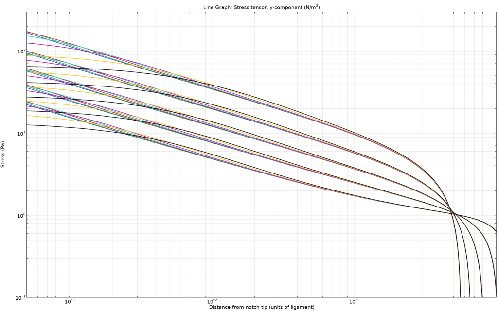
The same plot as shown above, but with the distance normalized by the ligament length.
The conclusion is that the constant slope regime for this case extends to about 10% of the ligament. Further away, the stress field is no longer controlled by the crack solution but by more global properties. How large this regime is for a certain geometry will depend on some length scale that is specific to that geometry.
Let’s investigate if the stress field in the crack solution can be used to predict the peak stress at the notch tip. We start by going back to the elliptical hole in a large plate. The ratio between the peak stress at an elliptical hole (with width a and notch radius R) and the stress intensity factor for a crack (with length a) is
If we assume that R << a, then the peak stress can be expressed in the stress intensity factor as
The idea is then that when a stress intensity factor can be computed, it’s possible to determine the stress at a rounded crack tip using an expression like
where the coefficient \beta is a configuration-dependent number of the order of 1. We can try this hypothesis on the example above.
In the plots below, the expression
is shown as a function of the notch depth, using the notch radius as the parameter. Two different geometries are used: the edge notch and a central slit. The latter case is obtained by adding a symmetry condition to the model.
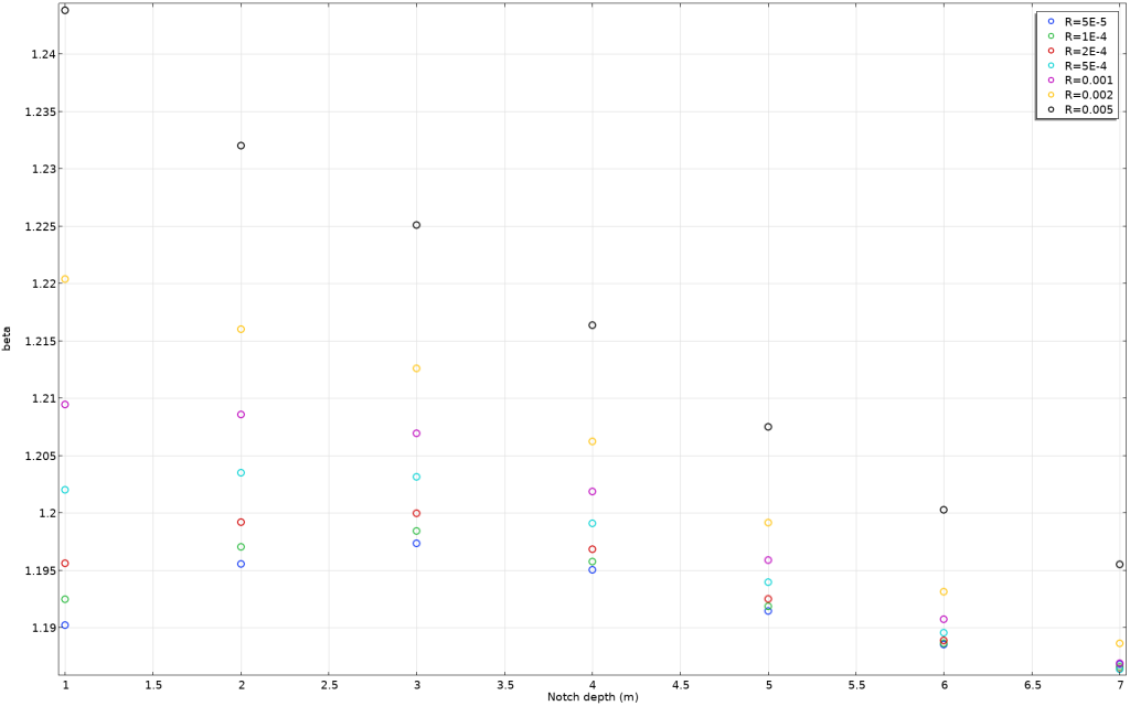
The factor \beta for the case with an edge notch.
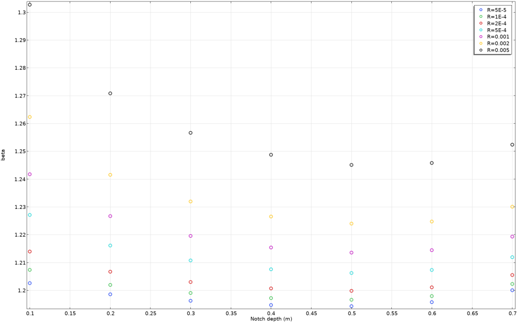
The factor \beta for the case with a central slit.
As can be seen, the actual value of the assumed multiplier \beta is close to 1.2 for both cases as long as the notch radius is small. For large notch radii and small notch lengths, the resemblance to a crack is not as good. The simplification using R << a is not valid.
To produce these graphs, the analytical value of K_I was used. In a real case when it’s not known, the solutions at a distance from the notch can be used to numerically determine K_I.
As a matter of fact, any sharp corner has a region where the stress field decays as r^{-p}, where r is the distance from the corner. So far, we have seen that the ideal crack has p = 0.5. The value of p for any opening angle is shown in the diagram below.
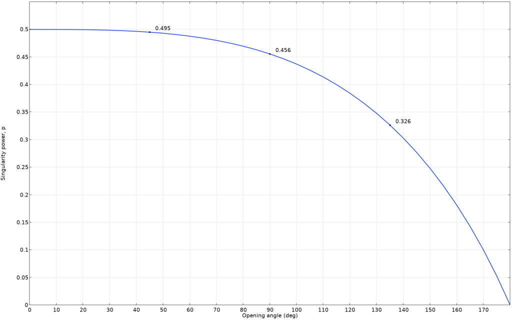
Power of the stress decay singularity for different opening angles. The values for 45°, 90°, and 135° are highlighted.
The curve was drawn by solving the transcendental equation \sin \left ((1-p)(2\pi-\alpha) \right) +(1-p) \sin(2\pi-\alpha) = 0, where \alpha is the opening angle.
For completeness, we can check the solution of the transcendental equation in an FE model of a strip in tension with an internal corner. The model is parameterized using the opening angle of the corner.
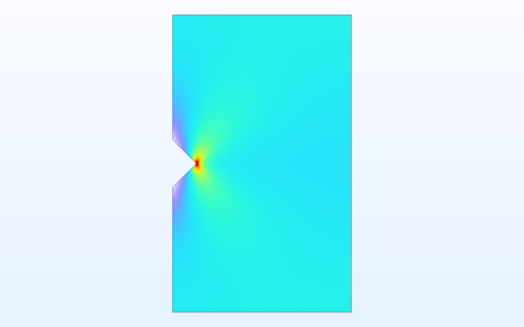
The von Mises stress in the model with the internal corner, for the case where the opening angle is 90°.
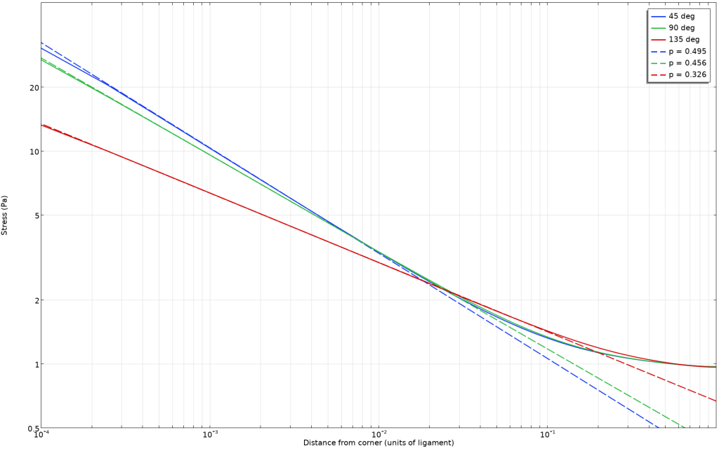
Vertical stress along the ligament. The distance from the tip of the corner is normalized by the ligament length. The dashed lines show the theoretical solutions, using the p-values from above.
As can be seen, there are regimes with almost straight lines in the stress-versus-distance diagram, which in the vicinity of the corner are in close agreement with the theoretical slopes.
Another type of singularity is caused by a material discontinuity. In practice, this often occurs together with a geometric singularity. We will limit the scope here to studying a pure material discontinuity in a bar subjected to tension.
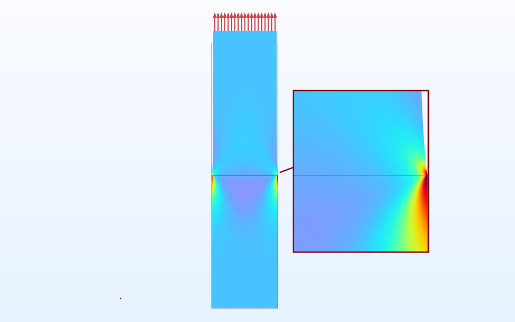
A bar where the lower part is stiffer than the upper part. The stress in the loading direction is plotted.
There are some general properties that can already be noted in this first plot:
- A singularity occurs on the free surface.
- The stress in the stiff material is higher than at the corresponding location in the softer material.
In order to examine this in more detail, we can create graphs showing the decay of the stress as a function of the distance from the material interface.
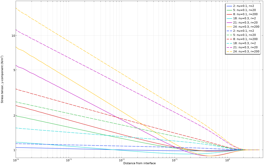
Stress in the loading direction plotted along the free boundaries as a function of the distance from the interface. The solid lines show the results in the soft material, while the dashed lines show the results in the stiff material. The parameter r is the ratio between the two Young’s moduli.
Again, we can identify straight lines in the log–log diagram, indicating that the stress varies with the distance as r^{-p}. The power ‘p’ is the same in both materials (solid and dashed lines of the same color are parallel). The strength of the singularity is controlled both by the ratio between the two elastic moduli and by the Poisson’s ratio values.
By looking at the (exaggerated) deformed shape in the surface plot above, this can be interpreted physically: The softer material will, for the same load, extend more than the stiffer material. That is, the strains in the load direction will become larger when in soft material. This also means that there will be a correspondingly larger contraction in the transverse direction, given that the two materials have the same Poisson’s ratio. This contraction will, however, be inhibited at the interface between the two materials, giving rise to the local stress singularity.
If we choose
then this singularity will disappear completely.
The conclusion is that a material transition will, in most cases, cause a singularity. Also, in this case, there is a region in the vicinity of the discontinuity where the stress decays according to a power law.
We have now studied the most common types of singularities that occur in FE modeling and have seen that they share a common property: The stresses in the vicinity of the singularity have a power-law dependence on the distance.
Weld Evaluation
Designing welds so that they are safe against fatigue is an important field in engineering. Much effort has been spent to provide systematic methods for predicting failure, even though accurate stress evaluation in general is impossible. In this case, it’s mainly the fact that the real geometry of the weld is unknown that causes the problem. Depending on the exact local geometry, the weld may or may not also introduce a stress singularity. To add further complexity, there are often hidden defects in the weld. The exception is when high quality is needed, in which case the weld may be ground and checked by some nondestructive testing method. But in most cases, it’s not meaningful to perform a detailed local stress analysis of the weld.
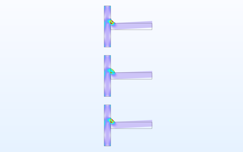
A fillet weld, but with three different local geometries.
An introduction to stress evaluation in welds is given in our blog post “How to Predict the Fatigue Life of Welds”.
Rather than digging into the details of weld analysis, it’s the design philosophy that is interesting here:
- Compute the stresses at a well-specified location, not at the weld toe itself.
- Establish allowed values for that stress. This must typically be done experimentally.
- The allowed stress value depends on how and where you have agreed to evaluate the stresses, so it’s not a true material property.
Back in the days when you did pen and paper calculations, all local effects were ignored. The allowed stress values had to account for that and were thus low. The modern FE-based approaches take part of the stress concentration into account (the part caused by the global geometry, but not the local weld geometry). The stresses can then be allowed to be higher but still significantly lower than what a pure material test would indicate.
In finite element terms, a shell model will typically return the stresses you are looking for, while a solid mechanics model will capture stress details that you don’t want when performing a fatigue analysis of welds.
Suggested Approaches
There are some fundamentally different reasons why your FE model may contain singularities. For instance:
- The boundary conditions induce singularities, as discussed in the blog post mentioned earlier. If such a singularity poses a problem for the analysis, it can be solved by refining the boundary conditions.
- A sharp corner is introduced because the local geometry has such a scale that it’s not reasonable to model a fillet at the global scale. In this case, there is no true singularity but rather a well-defined stress concentration. The most accurate approach is to use submodeling to determine the local stress state from the global solution. In the global model, you can use the amplitude of the power-law decaying stress field in the vicinity of the stress concentrations to know where to focus your efforts. Another possibility is to combine knowledge about the near-field stress field with knowledge about how it correlates to a local stress concentration to arrive at an estimate of that local stress concentration.
You can follow the pattern from weld evaluation but adapt it to your local conditions. In order to do that, you need a wide base of experience to build on. Which of the previous designs failed, and which did not? Then you need to analyze the previous designs and try to find an evaluation method that correlates with the experience.
Start by setting up FE models of these designs and try to identify a region where the stress or strain field is in the range where it’s neither controlled by the local notch details nor by the more global geometry. It may be necessary to use submodeling, at least while developing the criterion.
What criterion to use is usually not obvious. Since you are only going to perform relative comparisons, and not relate the computed number to any physical strength value, there are many possible choices. Here are some examples:
- The quantity should be easy to evaluate.
- The quantity should not be too sensitive to uncertainties in the analysis.
- If possible, the quantity should be physically relevant. For example, if the material is brittle, it may be better to look at the largest principal stress or principal strain than to use an equivalent stress criterion like von Mises.
- If fatigue is an issue, the quantity must be sensitive to load reversals.
- If possible, select a strain criterion rather than a stress criterion. The reason is that strains are computed directly from the displacements. The stresses are then computed using a combination of the strains. This means that a single inaccurate component in the strain tensor will propagate into all elements in the stress tensor.
- In the COMSOL Multiphysics® software, you can use the Safety feature to evaluate a large number of different criteria, including user-defined ones.
In a general case, the power of the singularity is not known. We do, however, know that in a certain region, the quantity of interest varies as
The values of K and p can be obtained by a least-squares fit or simply by using the values in two points on the part of the line that is straight in a log–log diagram. Since p must be considered as property that is constant for a certain type of singularity, the computed value can be used as a check on the validity of the approach.
With p known, it’s the value of K for a certain configuration that should be compared with an allowed value. This is in analogy how cracks are treated in fracture mechanics.
The Percentile Method
Another approach for obtaining an allowed stress level is to define a reference stress as the value that is exceeded in a given fraction (for example, 5%) of a reference volume. If this reference stress is lower than the allowed value, the design is accepted. By using this approach, the problem with evaluations close to the singularity is avoided. It’s only essential to be able to compute the volume where the reference stress is exceeded, and the boundary of that volume will be at some distance away from the singularity, where the solution is well converged.
This method seems simple, but it requires quite some standardization in order to be applied. One problem here is how to determine the reference volume. If the total volume of the structure is used, it will be possible to decrease the reference stress just by adding more material in a low-stress region, which of course does not make sense. The reference volume must be related to, for example, the size of a specific region around the singularity. Another drawback is that optimization methods may choose to relocate stresses so that the reference stress is decreased while the peak stress is increased.
Again, it’s only possible to compare similar structures with each other.
Now, let’s discuss how to evaluate the stress value using the percentile method. In COMSOL Multiphysics®, it’s not possible to directly evaluate the 5% stress value. Three alternative methods are described below.
Method 1
If only a single evaluation is needed, the fastest option is usually to do a few manual iterations. You just create an integration operator (say, intop1) and evaluate an expression like intop1(solid.mises>sRef)/intop1(1). By changing the reference stress, sRef, a few times, you will soon find the value that corresponds to the given percentile.
Method 2
Use a model method to automate Method 1.
Method 3
You can set up an extra equation and solve for the stress value, as will be explained below.
The equation to be solved is the following:
Here, \sigma_\mathrm{c} is the computed stress. It may be an equivalent stress like von Mises, a first principal stress, or something else. It would, of course, be possible to use the same procedure for a strain or energy criterion. The reference volume is denoted V_\mathrm{ref}, and \beta is the percentile. The boolean expression inside the integral is assumed to evaluate to 1 where it’s true and to 0 where it’s false.
In order to get a scaling that is easier to handle for computations, it’s better to rewrite the equation as
The integral can be computed using an integration operator, as done in the first method. A straightforward way of implementing this equation using a Global Equation node is shown below:
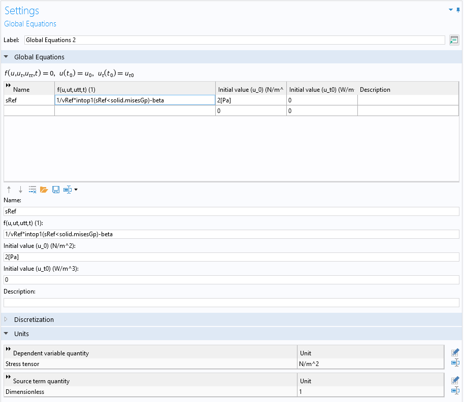
Unfortunately, this will not work. An inequality is not differentiable, so no Jacobian can be formed. The stiffness matrix will just contain zeros for this equation. It is possible, however, to circumvent this problem by introducing a manual finite difference derivative. The expression is lengthy, and requires some understanding of equation-based modeling in COMSOL®, so a detailed explanation is given in the Additional Info section below.
Below is a modified global equation that will solve the problem of finding the stress that gives the intended percentile.
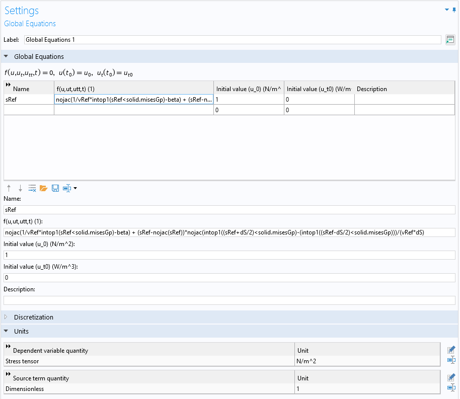
Here, the user-defined parameter dS is a stress increment, denoted by \Delta \sigma in the Additional Info section.
As an example of this approach, the same notched plate example from earlier is used. Since the reference volume should be independent of the size of the plate, we can, for example, choose a circle around the notch. In this case, the radius of the circle can be selected based on the following characteristic lengths of the structure:
- Width: 1 m
- Minimum crack length: 0.1 m
- Minimum ligament width: 0.3 m
- Maximum notch radius: 0.01 m
A reference volume based on a circle with the radius 0.05 m around the notch tip will be far from the boundaries of the structure, but also far from the details of the notch itself.
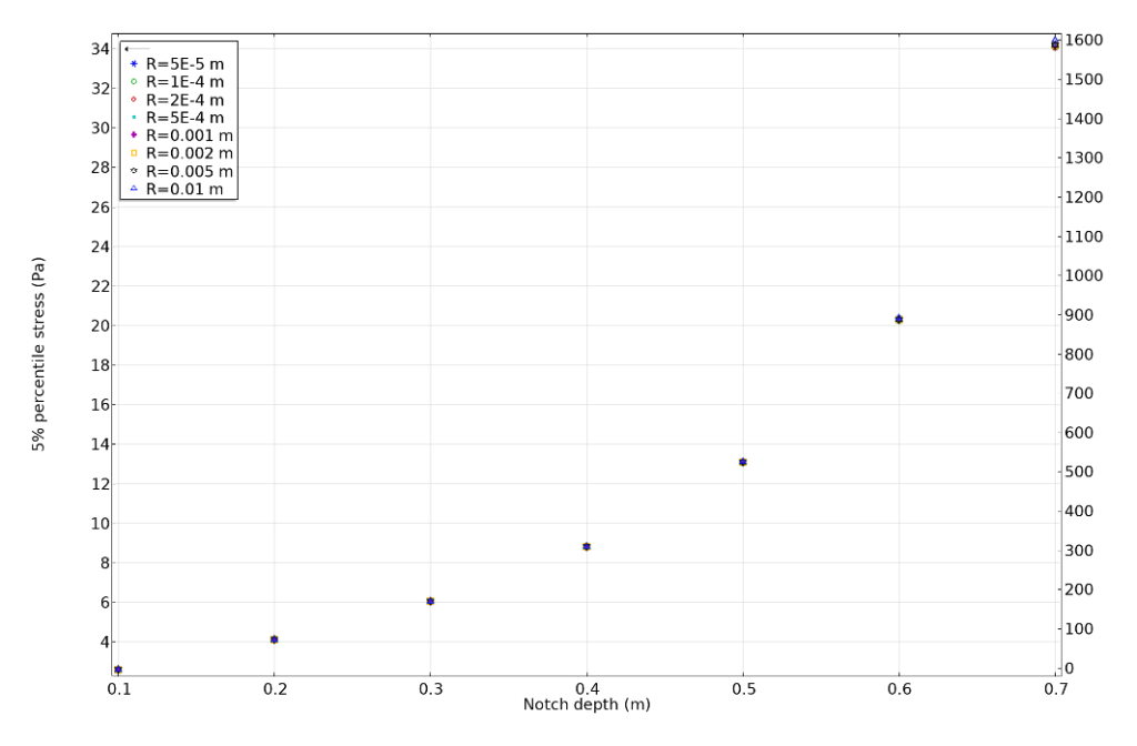
The stress level that is exceeded in 5% of the reference volume for different values of the slit depth and notch radius.
For all values of the slit depth, the 5% percentile stress is essentially independent of the notch radius. It’s only sensitive to the slit depth. This is in line with the underlying idea: Avoid sensitivity to the details of a local, possibly singular, stress field. The same result is obtained irrespective of whether a sharp tip or a fillet is used. Essentially, this approach gives the same information as the stress intensity factor: it measures the intensity of the singularity. If structures with the same type of fillet are compared, this method could provide a suitable criterion.
Additional Info
The expression contains two terms: The first one creates the residual, and the second one creates the Jacobian. This is a solution that generally can be used in advanced modeling. If, for example, an exact Jacobian is expensive to create, you can use similar expressions to form a correct residual together with an approximate Jacobian.
The nojac(expr) operator, which is used in several places, ensures that no Jacobian contributions are generated for the given expression.
The Jacobian term is multiplied by the factor (sRef-nojac(sRef)). Since this expression always evaluates to zero, no residuals will be generated from that part of the expression. The derivative of sRef with respect to itself is simply 1, and the remainder of the expression is a symmetric finite difference expression of the derivative,
Here, \Delta \sigma is a finite change in the stress. It should be chosen to be as small as possible while still having the property that the volume computed by \displaystyle \int_V (\sigma_\mathrm{ref}+\Delta \sigma<\sigma_\mathrm{c}) \; dV differs significantly from \displaystyle \int_V (\sigma_\mathrm{ref}<\sigma_\mathrm{c}) \; dV . A good level is when the change in stress over one element is \Delta \sigma in the vicinity of the isosurface for the resulting reference stress \sigma_\mathrm{ref}.
Concluding Remarks
Even though it is impossible, from a theoretical perspective, to evaluate gradients and fluxes (strains and stresses) at a singularity, there are systematic methods by which you can approach the problem. Such methods do, however, require that you have enough experimental evidence to interpret a judiciously chosen critical quantity.
To download the models used in this blog post, click the button below.

Comments (0)