

Welcome back to our discussion on multiscale modeling in high-frequency electromagnetics. Multiscale modeling is a simulation challenge that arises when there are vastly different scales in a single simulation, such as the size of an antenna compared to the distance between the antenna and its target. Today, in Part 4 of the series, we will examine how we can construct a multiscale model by coupling a Full-Wave antenna simulation with a geometrical optics simulation using the Ray Optics Module.
Using the Ray Optics Module for Multiscale Modeling
In Part 2 of the blog series, we used the Electromagnetic Waves, Frequency Domain interface, which we call a Full-Wave simulation, and a Far-Field Domain node to determine the electric field in the far field. We then coupled a Full-Wave simulation to the Electromagnetic Waves, Beam Envelopes interface (or a Beam-Envelopes simulation) in order to precisely calculate fields in any region, regardless of the distance from the source.
The Far-Field Domain and Beam-Envelopes solutions that we looked at in the previous blog post are effective, but they share one noteworthy restriction. In each case, we assumed that a homogeneous domain surrounded the antenna in all directions. For many situations, this information is sufficient. In other simulations, you may not have a homogeneous domain surrounding your antenna and you need to account for issues like atmospheric refraction or reflection off of nearby buildings. These simulations require a different approach.
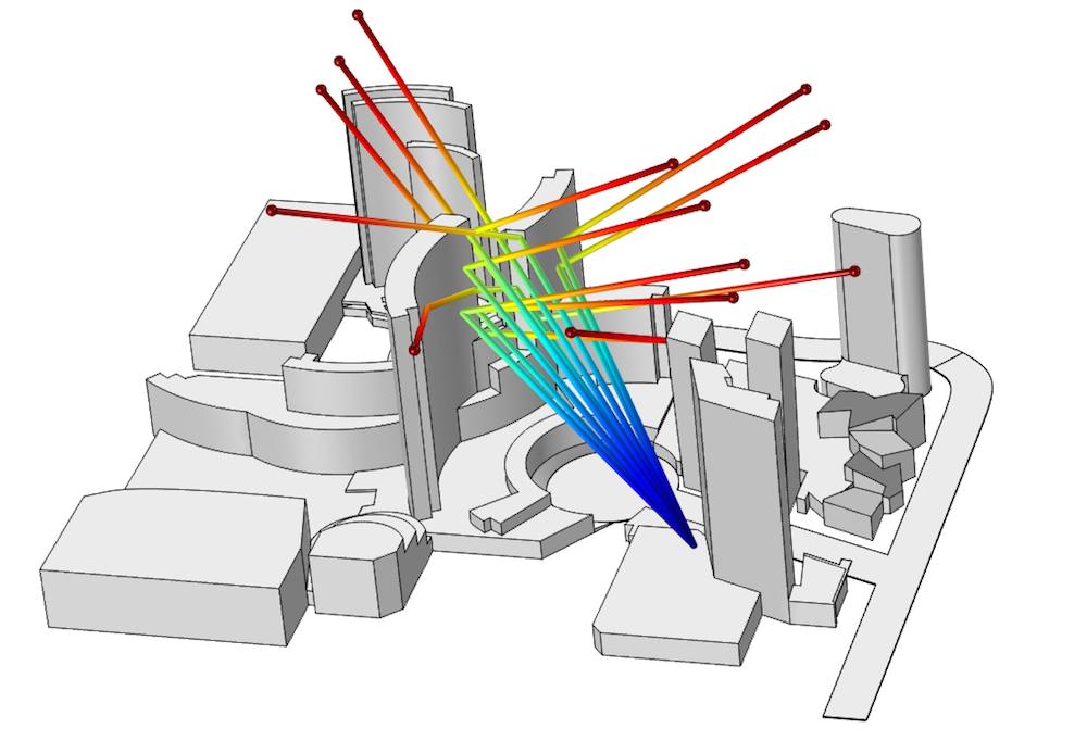
A model of several hotels in Las Vegas. A directional antenna emits rays toward the ARIA® Resort & Casino.
The Geometrical Optics interface in the Ray Optics Module, an add-on product to the COMSOL Multiphysics® software, regards EM waves as rays. This interface can account for spatially varying refractive indices, reflection and refraction from complicated geometries, and long propagation distances. However, these features come with a tradeoff. Since waves are treated as rays, this approach neglects diffraction. In other words, we are assuming that the wavelength of light is much smaller than any geometric features in our environment. You can read a more thorough description of ray optics in a previous blog post.
Modeling Coupled Antennas: Preparing for Ray Optics
As you may recall, we introduced an approach to coupling a radiating and receiving antenna in Part 3 of this series. When incorporating ray optics into our multiscale modeling, we are required to use a similar but more generalized approach. Before we show you how to set up a geometrical optics simulation in COMSOL Multiphysics, let’s first review this alternate method.
Mapping the Radiated Fields
As a quick refresher, we are interested in calculating the fields at the location of the receiving antenna using the following equation:
We previously used an integration operator on a single point to calculate this along the line directly between the two antennas. We now wish to retain the angular dependence, so we need to recalculate this equation for each point in the receiving antenna’s domain. Since it is impractical to add numerous points and integration operators, we need to establish a more general technique.
To do so, we replace the integration operator with a General Extrusion operator. As before, we create a variable for the magnitude of r. We then use the General Extrusion operator to evaluate the scattering amplitude at a point in the geometry that shares the same angular coordinates, (\theta,\phi), as the point in which we are actually interested.
To demonstrate this concept, we use a figure that is slightly more involved than that from the previous post. Note that the subscripts 1, 2, and r in \vec{r}_j=\left(x_j,y_j,z_j\right) represent a vector in component 1, a vector in component 2, and the offset between the antennas, respectively.
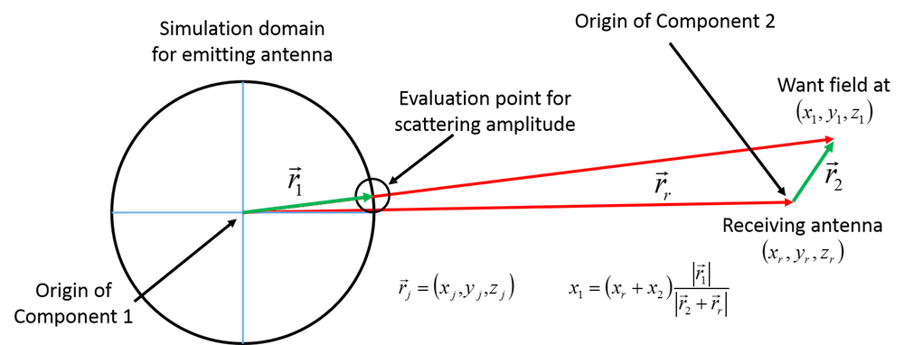
Image showing where the scattering amplitude should be calculated and how the coordinates of that point can be determined.
As we previously outlined, the primary complication is determining where to calculate the scattering amplitude. We want the fields at the point \vec{r}_r + \vec{r_2}, which requires calculating the scattering amplitude at \vec{r}_1. The complication, of course, is that each point in the domain around the receiving antenna (each vector \vec{r}_2) will have its own evaluation location \vec{r}_1. We evaluate this by again rescaling the Cartesian coordinates, but instead of doing it for a single point, we define it inside of the general operator so that it can be called from any location. From the above figure, we know that this point is x_1 = \left(x+x_r\right) \frac{|\vec{r}_1|}{|\vec{r}_2+\vec{r_r}|}, with corresponding equations for y and z. The operator is defined in component 1, so the source will be defined in that component. It will be called from component 2, so the x, y, z in the following expressions refer to x2, y2, z2 in the above figure.
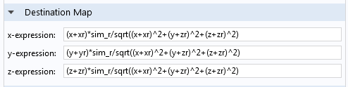
The General Extrusion operator used for the scattering amplitude calculation. Note that this is defined in component 1.
Storing the Radiated Fields in a Dummy Variable
As a bookkeeping step, we store the calculated fields in a “dummy” variable. By a dummy variable, we mean that we add in an extra dependent variable that takes the value of a calculation determined elsewhere. We do this for two reasons.
The first reason is that most variables in COMSOL Multiphysics are calculated on demand from the dependent variables. In an RF simulation, for example, the dependent variables are the three Cartesian components of the electric field: Ex, Ey, and Ez. These are determined when computing the solution. In postprocessing, every other value (electric current, magnetic field, etc.) is calculated from the electric field when required. In most cases, this is a fast and seamless process. In our case, each field evaluation point requires a general extrusion of a scattering amplitude, and each scattering amplitude point requires a surface integration as defined in the Far-Field Domain node. This can take a while and we want to ensure that we perform this calculation only once.
The second reason why we do this has to do with the element order. The Scattered Field formulation requires a background electric field. COMSOL Multiphysics then calculates the magnetic field using the differential form of Faraday’s law (also known as the Maxwell-Faraday equation). This requires taking spatial derivatives of the electric field. There are no issues when taking the spatial derivatives of an analytical function like a plane wave or Gaussian beam, but it can cause a discretization issue when applied to a solved-for variable. This is a rather advanced topic, which you can find out more about in an archived webinar on equation-based modeling.
By using a cubic dummy variable to store the electric field, we can take a spatial derivative of the electric field and still obtain a well-resolved magnetic field for use in the Scattered Field formulation. Without the increased order of the dummy variable, the magnetic field used would be underresolved. Below, you can see what it looks like to put the General Extrusion operator together with the dummy variable setup. The variable r is identical to the one used in Part 3 of this blog series and is defined in component 2.
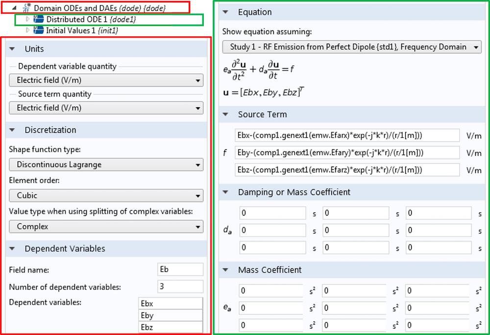
The dummy variable implementation. Notice that the dummy variable components are called Ebx, Eby, and Ebz.
The only remaining step is to use the dummy variables — Ebx, Eby, and Ebz — in a background field simulation of the half-wavelength dipole discussed in Part 1 and Part 3.
This technique isn’t actually very good for this particular problem. There may be situations where it is useful, but the technique from Part 3 is preferred in the vast majority of cases. The received power from the two simulations is extremely close, but this method takes much longer to calculate and the file size increases drastically. In the demo examples for this post, this method took several times longer than the previous simulation method. While you may conclude that this is not a terribly useful step overall, it is useful when we incorporate ray optics into our multiscale modeling, as discussed in the next section.
Setting Up a Geometrical Optics Simulation in the COMSOL® Software
A geometrical optics simulation implicitly assumes that every ray is already in the far field. Earlier in the blog series, we saw that the Far-Field Domain feature correctly calculates the electric field at arbitrary points in the far field. Here, we use that information as the input for rays in a geometrical optics simulation. The simulation geometry, symmetry, and electric dipole point source used are the same as in Part 2.
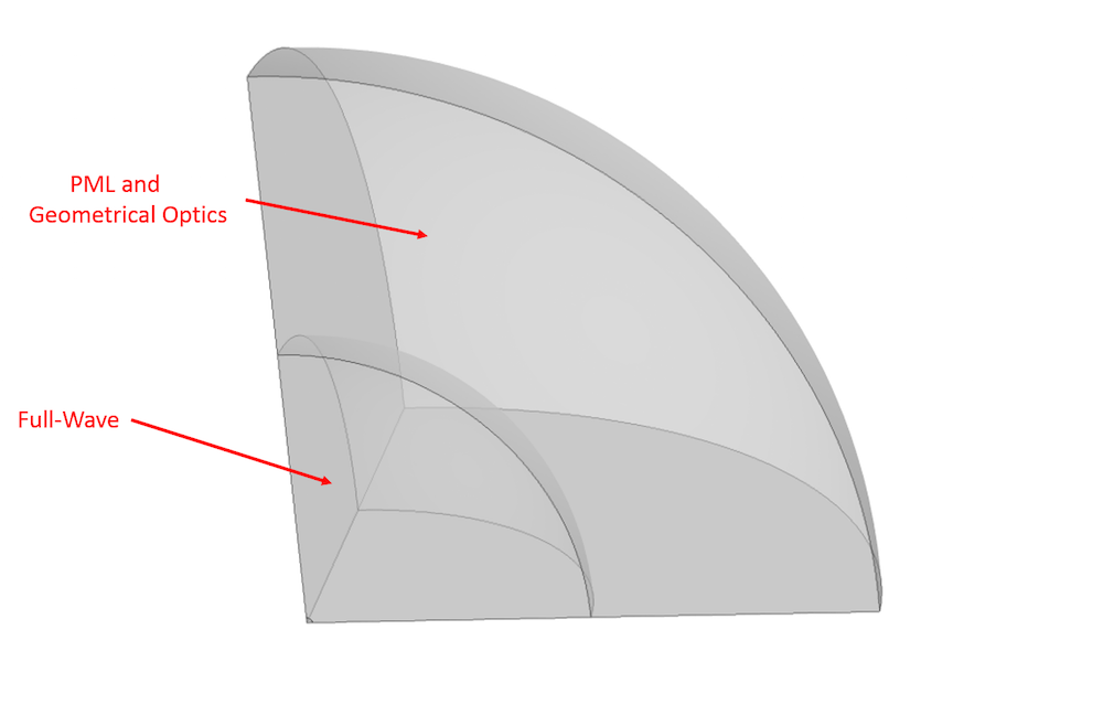
The domain assignments for the simulation. The Full-Wave simulation is performed over the entire domain, with the outer region set as a perfectly matched layer (PML). The geometrical optics simulation is only performed in this outer region. Note that this image is not to scale.
With the domains assigned, we select the Geometrical Optics interface, change the Intensity computation to Compute intensity, and select the Compute phase check box. These steps are required to properly compute the amplitude and phase of the electric field along the ray trajectory.
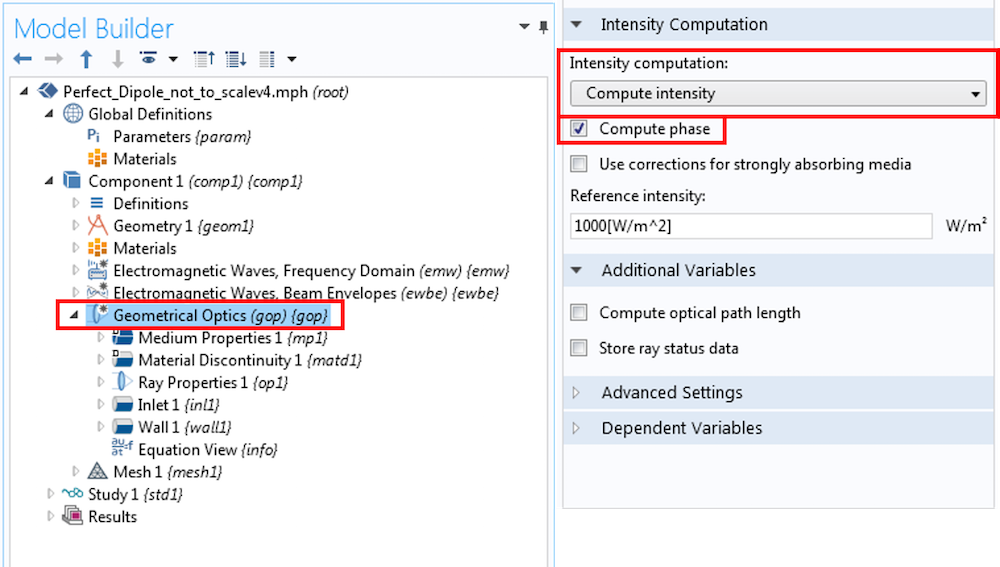
Settings for the Geometrical Optics interface. The Intensity computation is set to Compute intensity and the Compute phase check box is selected.
We also apply an Inlet boundary condition to the boundary between the Full-Wave simulation domain and Geometrical Optics domain. The inlet settings can be seen in the image below, but let’s walk through them one at a time. First, the Ray Direction Vector section is configured. This will launch the rays normal to the curved surface we’ve selected for the inlet — in other words, radially outwards. The variables Etheta and Ephi are calculated from the scattering amplitude according to
with a similar assignment for Ephi.
This equation comes from our previous blog post about using the Far-Field Domain node to calculate the fields at an arbitrary location. These variables are used to specify the initial phase and polarization of the rays. The GOP\_I0 variable specifies the correct spatial intensity distribution for the rays (as antennas generally do not emit uniformly) and is calculated according to GOP\_I0 = (|Etheta|^2 + |Ephi|^2)/Z/2, where Z is the impedance of the medium.
The initial radius of curvature has two factors. The parameter dipole\_sim\_r is the radius of the spherical boundary that we are launching the rays from and will correctly initialize the curvature of the ray wavefront.
Finally, we use the Cartesian components of our spherical unit vector \hat{\theta} to specify the initial principal curvature direction. This ensures that the correct polarization orientation is imparted to the rays. The wavefront shape here must be set to Ellipsoid — even though the surface is technically a sphere — because we need to be able to specify a preferred direction for polarization. If we choose Spherical, then each orientation is degenerate and we cannot make that specification.

The settings for the Inlet boundary condition in the Geometrical Optics interface. Note that you can click the image to expand it.
Beyond setting the correct frequency, the only other setting here is the placement of a Freeze Wall condition on the exterior boundary to stop the rays. Let’s take a look at the results vs. theory. As before, we express the full solution for a point dipole as a sum of two contributions, which we have labeled near field (NF) and far field (FF).
\overrightarrow{E} & = \overrightarrow{E}_{FF} + \overrightarrow{E}_{NF} \\
\overrightarrow{E}_{NF} & = \frac{1}{4\pi\epsilon_0}[3\hat{r}(\hat{r}\cdot\vec{p})-\vec{p}](\frac{1}{r^3}+\frac{jk}{r^2})e^{-jkr}\\
\overrightarrow{E}_{FF} & = \frac{1}{4\pi\epsilon_0}k^2(\hat{r}\times\vec{p})\times\hat{r}\frac{e^{-jkr}}{r}\\
\end{align}
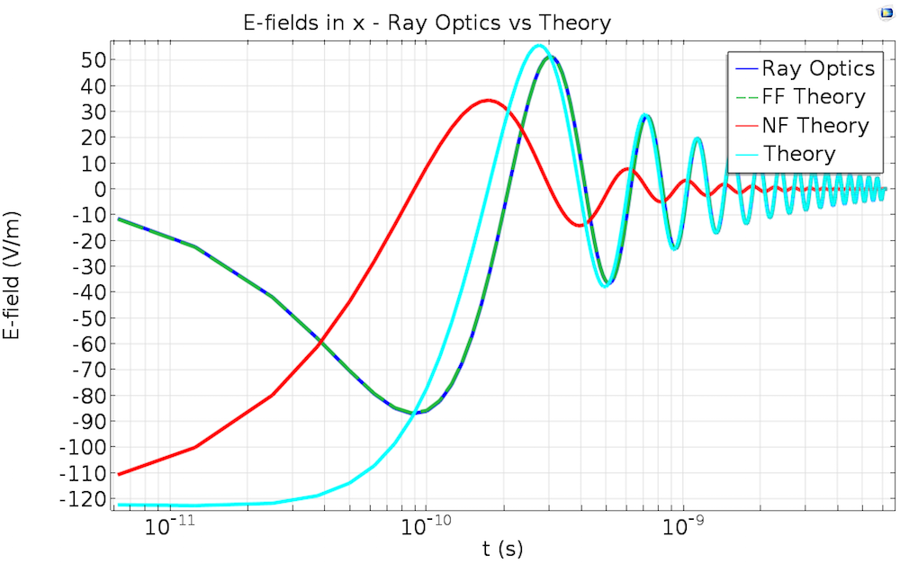
The electric fields from a geometrical optics simulation compared against theory. Geometrical optics is always in the far field, so we see excellent agreement as the distance from the source increases. For reference, the far-field domain results from the previous post would overlap exactly with the ray optics and FF theory lines.
As mentioned before, the Geometrical Optics interface is necessarily in the far field, so we do not expect to be able to correctly capture the near-field information as we did in the Beam-Envelopes solution in Part 2. This can also be seen because we seeded the ray-tracing simulation with data from the Far-Field Domain node calculation. It is therefore unsurprising that there is disagreement near the source, but we can clearly see that the results match with theory as the distance from the source increases.
Summary of Multiscale Modeling Techniques
From looking solely at the above plot, we have to ask ourselves: “What have we actually gained here?”
This is a fair question, because the plot shown above could have been constructed directly from any of the techniques covered in the series so far. To make this clear, let’s review each of them.
| Multiscale Technique | Regime of Validity | Modules Used | Notes |
|---|---|---|---|
| Far-Field Domain node | Far field | RF or Wave Optics | Requires the antenna to be completely surrounded by a homogeneous domain. |
| Beam-Envelopes | Any field | Wave Optics | Requires specification of the phase function or wave vector. |
| Geometrical Optics | Far field | Ray Optics | Can account for a spatially varying index as well as reflection and refraction from complex geometries. Diffraction is neglected. |
A summary of the multiscale modeling techniques we have covered in this blog series.
Note that any of these techniques will require a Full-Wave simulation of the radiation source. This generally requires the RF Module, although there is a subset of radiation sources that can be modeled using the Wave Optics Module instead. The Far-Field Domain node is available in both the RF and Wave Optics modules.
We originally motivated this discussion by talking about signal transmission from one antenna to another, and solved that simulation using the Far-Field Domain node in the last post. In the next blog post in this series, we’ll redo that simulation using the Geometrical Optics interface introduced here.
Access the model discussed in this blog post and any of the model examples highlighted throughout this blog series by clicking on the button above.
ARIA is a registered trademark of CityCenter Land, LLC.

Comments (0)