COMSOL Blog

Examining an Air Filter with a RANS Turbulence Model

February 20, 2024

HVAC systems do more than provide the smooth, chilled air that flows when the temperature outside rises. Within these systems, air moves through filters to ensure high air quality. With clean air at stake, modeling and simulation can be used to gain an in-depth understanding of the physics behind the behavior of air as it moves through a filter…

Modeling an Air Filter

The filters within HVAC systems rely on a material (often fiberglass or cotton folds) capable of straining the air and catching particulates like dust, pollen, and bacteria. These materials impact the flow of the air, catching the unwanted particulates while simultaneously allowing the filtered air to flow through. Modeling these devices and the turbulent flow they induce allows for determining the effectiveness of different materials when they are used for filters, helping designers to narrow down the material options before investing in real-life, experimental versions.

In this blog post, we will look at a common air filter geometry (shown below) as our example.

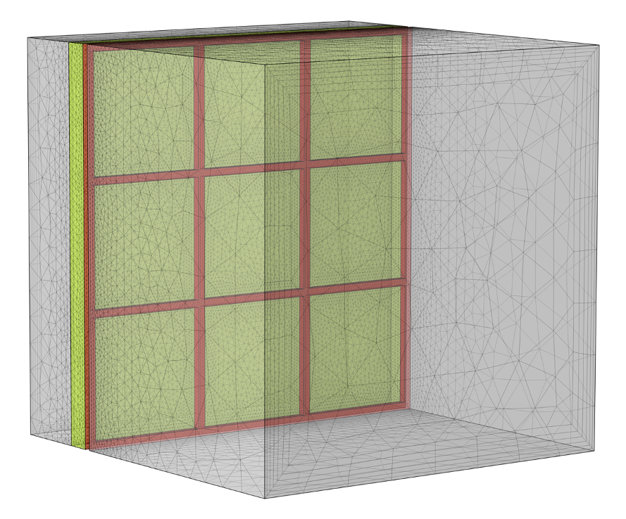
A mesh of the air filter and open fluid domains, where the filter is more densely meshed than the domains.
Model geometry showing the inlet section and the longer outlet section with the filter placed in between. The filter geometry is more densely meshed than the open fluid domains.

Modeling this air filter begins with the CFD Module, an add-on product to the COMSOL Multiphysics^® software, which enables users to create Reynolds-averaged Navier–Stokes (RANS) turbulence models in open and porous domains. In this example, the air filter is modeled as a highly porous domain with 90% of the material occupied by cylindrical pores with a diameter of .1 mm. The support of the air filter is represented by a frame with no-slip walls. For this example, we employed the Turbulent Flow, k-ω interface because of its accuracy for models with many walls, including no-slip walls. (An in-depth look at the model setup can be found in the model documentation, which can be accessed via the button at the end of this blog post.)

Evaluating the Results

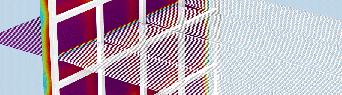
Solving the model allows for visualizing the change in turbulence, velocity, and pressure as air moves toward, through, and past the filter. The computation begins with the air moving toward the filter (purple in the image below). When the air passes through the filter, the interstitial velocity increases (although the porous-averaged velocity remains constant), resulting in an increase in turbulence kinetic energy. Additionally, there is an abrupt pressure drop due to the increase in velocity and the increased friction and pressure losses, which stem from the high number of wall surfaces. As for the behavior of the air as it moves away from the filter, the frame of the filter prevents the air from moving freely, instead causing downstream wakes of air.

Plot showing the velocity magnitude at the inflow surface of the air filter.
The pressure significantly decreases across the porous air filter.

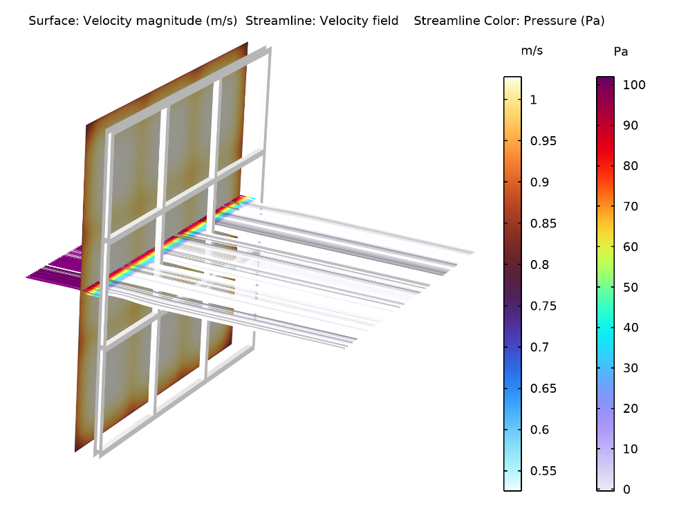
The visualization of the air moving through the filter can be used to conclude whether or not the filter will remove contaminants from the air. To confirm this conclusion, the solution can be evaluated with different slice plots. One of the slice plots for this example indicates that the velocity of the air is most impacted by the porous air filter and the frame and that it homogenizes through the wake region. A slice plot measuring the turbulence kinetic energy shows that the turbulence kinetic energy peaks noticeably within the filter and attains typical values on the no-slip walls.

In general, the model points to a pressure drop and a dramatic increase in turbulence within the filter, creating perturbations in velocity perpendicular to the main direction of the flow thus also increasing the probability of the particles to collide with the pore walls and stay there. In other words, the increase in turbulence provides the mixing required for filtering out the unwanted particulates, which otherwise would flow through the pores undisturbed.

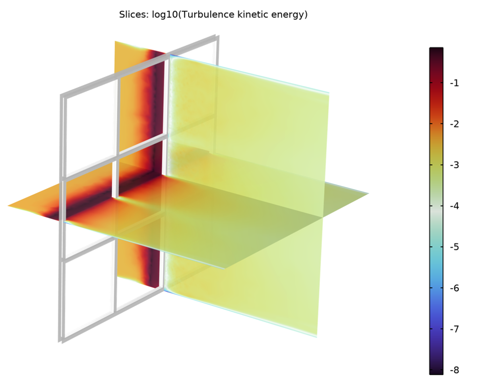
A slice plot showing the horizontal and vertical slices of the turbulence kinetic energy, which highlights that the porous domain produces k values several orders of magnitude higher than the values upstream and downstream.
A slice plot showing the turbulence kinetic energy. The turbulence level is significantly higher in the porous air filter than in the free stream or near the duct walls.