
One of the challenges in the field of inductive heating is the modeling of the nonlinear properties of the materials being heated. All materials are nonlinear with temperature; magnetic materials are also nonlinear with magnetic field. Incorporating these nonlinearities into a model is necessary for accuracy. Here, we will look at one particularly convenient way to do so using the Magnetic Field Formulation interface within the AC/DC Module, an add-on to the COMSOL Multiphysics® software.
Why Induction Heating is a Modeling Challenge
Induction heating is widely used in materials processing applications for many reasons, including:
- The workpiece is indirectly heated.
- The zone being affected can extend into the volume of the material.
- The heating profile over time can be very precisely controlled by altering the magnitude and frequency of the driving currents.
Precise control over the heating process, however, does require some kind of process feedback loop and experimental verification. This loop should ideally be augmented with a numerical model that incorporates experimental data and can predict the temperature evolution over time. A numerical model is especially useful since it can predict behavior in regions that are not directly measurable in real time.
Practically speaking, numerical models do pose several challenges. You need good input data, starting with an accurate description of the geometry of the workpiece and induction heating coil, as well as knowledge of the driving currents and frequencies. From there, you also need to know the material properties and how they vary.
All material properties vary with temperature, and since induction heating usually starts with the workpiece at around room temperature and raises it up to around the melting temperature, these nonlinearities can never be neglected. Both the electrical and thermal conductivity of metals usually decrease with increasing temperature, but not always.
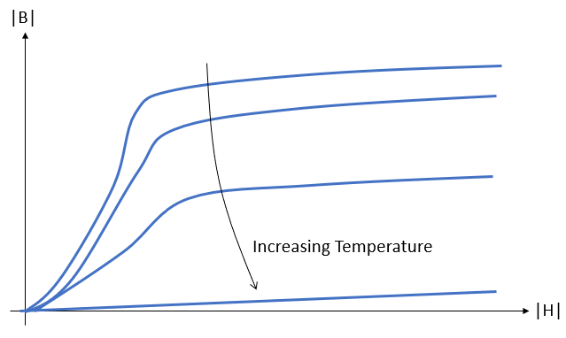 Representative B–H curves at different temperatures. Above the Curie temperature, the slope of the curve equals the magnetic permeability of free space.
Furthermore, there are some materials, specifically soft magnetic materials, that have magnetic permeability that is nonlinear with magnetic field but with neglectable hysteresis. These materials can be experimentally characterized by a B–H curve, relating the magnitude of the \mathbf{B}-field to the \mathbf{H}-field. These curves also exhibit a change with temperature, decreasing gradually in magnitude up to the Curie temperature, at which point the material becomes nonmagnetic. Although the form of such curves will usually be quite similar to what is shown above, the actual experimental data can be difficult to acquire and will often represent the biggest hurdle to implementing a numerical model.
Implementing the Model: A Few Conceptual Preliminaries
Induction heating processes usually occur over a timespan lasting at least a few seconds, while the excitation frequencies can range from as low as 50 Hz up to 450 kHz or even beyond. This means that there are two temporal scales to the problem. The temperature fields can be assumed to vary quite slowly relative to one period of oscillation. In other words, the electromagnetic fields do not observe a variation in temperature over one cycle. This motivates a solution method termed the Frequency-Transient study approach, where the electromagnetic fields are solved in the frequency domain, while the thermal problem is solved in the time domain.
The electromagnetic fields do get recomputed but only when the material properties vary with respect to a change in temperature. The explicit assumption of a frequency domain analysis is that the material properties are constant over one cycle. However, in practice, the electromagnetic fields usually do vary nonlinearly over one cycle. We are usually trying to heat the material as quickly as possible, meaning that the excitation currents and resultant fields will be driving the material into the nonlinear part of the B–H curve.
To resolve this apparent contradiction, we use the concept of the effective B–H curve, which uses an energy-based method to compute a curve that approximates the nonlinear behavior. These curves can be computed by starting with the experimental tabulated B–H curve. The workflow begins with acquiring the B–H data, cleaning it up using the B–H curve checker, and then using the smoothed data within the effective B–H curve calculator.
Following the above concepts, you should now have at least three sets of data for the workpiece material:
- temperature
- nonlinear electrical and thermal conductivity
- a set of effective B–H curves at different temperatures for each material being heated
To set up a complete thermal model, you will also need the density and the specific heat, as well as the thermal emissivity of the surface since we will always need to consider at least radiative cooling. The specific heat also always varies with temperature. Density is always held constant — any change in volume has to be modeled by also solving for thermal expansion of the solid material. The surface emissivity is held constant in the example we will look at, although in practice it may vary.
The inductive coils are almost always water-cooled copper pipes and thus are much simpler to model since their temperature is fixed. We are usually not interested in the heat distribution within the coil itself. We only need to know how the currents in the coil are heating up the workpiece. This leads to a simpler modeling approach of using the Impedance Boundary Condition to model only the coil surface, thus avoiding the need to mesh the interior volume of the coil. This simplification can be relaxed by modeling the volume of the coil as well, if desired.
The workpiece, on the other hand, must always be modeled as a volume, since the variations in the properties cannot be accurately modeled via a surface condition. Furthermore, the fields will often vary quite sharply in the direction normal to the surface but quite gradually in the tangential direction. This motivates the usage of a boundary layer mesh. When working in 3D, it can even be useful to partition the geometry by introducing layers at the surface.
A Quick Aside: Using Analytic Equations for the Effective B–H Curve
Although experimental data is the ground truth, it is not always easy to acquire this data to high accuracy, especially over a wide temperature range. So, sometimes it motivates to use simpler expressions for the B–H curve, especially when we can use these to subsequently come up with analytic expressions for the effective B–H curve.
Two convenient expressions for the magnitude of the \mathbf{B}-field, B = \lVert \mathbf{B} \rVert, as a function of the magnitude of the \mathbf{H}-field, H = \lVert \mathbf{H} \rVert, are:
These have the same limiting behavior: at low magnetic field, the slope (the differential relative permeability) is \partial B / \partial H = \mu_{rd} = \mu_0\left( 1+B_{sat}/H_0 \right), and in the high-field limit, the slope is \mu_0, equal to free space. The saturation flux density, B_{sat}, is the point at which the slope approaches the free space limit.
By using this form, we can easily introduce a temperature dependency to approximate the behavior as we approach the Curie temperature, above which materials can be approximated as being nonmagnetic. We do so by making the saturation flux density a function of temperature, where the function B_{sat}\left(T\right) can have any form as long as it drops to zero above the Curie temperature. Usually, it will be monotonically decaying, so we could posit a curve of the form shown in the plot below, with polynomial decrease up to the Curie temperature. Such a curve can be defined using the Piecewise function in COMSOL®, and a smoothing term can be added for numerical stability.
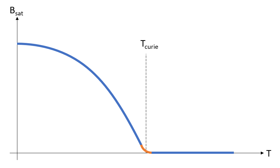 Approximation of the change of the magnetic behavior with temperature. Smoothing is applied over a small region about the Curie temperature.
With these expressions, we can now derive an analytic expression for the effective B–H curve using the Simple Energy method, where:
Plugging in our two expressions from above gives:
Note that we could also introduce a temperature dependency to the H_0 term, altering both magnitude and slope of the B–H curve. It should be emphasized that these are solely presented as convenient approximations, and you could repeat this derivation for other functions and other equations for computing the effective B–H curve. In the absence of high-quality experimental data, these can be a reasonable starting point for your modeling.
Implementing a Model Using the Magnetic Field Formulation
The case we will consider here is of a steel square channel heated by a three-turn coil. We will assume that the coil pitch does not strongly affect the solution and will use this assumption to exploit the symmetry of the workpiece and coil to reduce model size.
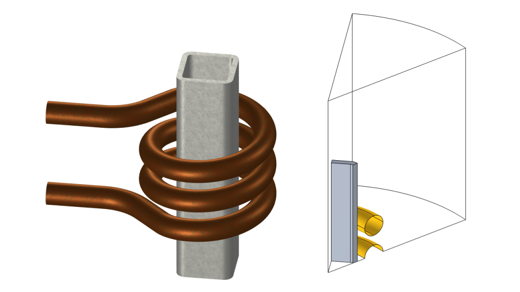 A three-turn inductive coil around a section of a steel square channel (left) can be reduced to a one-sixteenth model (right) of the workpiece and the surrounding free space.
The approach that we will take here is to use the Magnetic Field Formulation interface, which solves for the \mathbf{H}-field directly. This makes it slightly more suitable for modeling of materials where the nonlinearity depends explicitly on the \mathbf{H}-field itself. We’ve already covered how to introduce excitations into this formulation and will use a global constraint to fix the driving current on the coil.
When entering the material nonlinearity, you can reduce the computational cost by avoiding symbolic differentiation with respect to magnetic field in the effective B–H material relationship. This is done using the nojac () operator, and although this can occasionally lead to an increased number of solver iterations, each iteration takes less time and memory, resulting in an overall improvement. Note that this holds, regardless of whether you’re using the analytic expressions derived above or using tabulated data.
The solution approach uses the Frequency-Transient solver, which will default to using a segregated approach for 3D models. The \mathbf{H}-field is solved for using a direct solver, and this is a great place to try out the new NVIDIA CUDA® direct sparse solver (NVIDIA CuDSS) if you have an appropriate graphics card.
The results are animated below, and show the effects of the rise in temperature. The effective relative permeability changes as the part heats up, and eventually drops to unity once the Curie temperature is exceeded.
Animation of the effective relative permeability, which is affected by field strength and temperature, over time.
With regards to the meshing, you can use the maximum operating frequency along with the conductivity and maximum effective permeability to compute the minimum skin depth. Along with that, you can investigate different element order, although when you have highly nonlinear materials, the linear order is usually preferred.
The computational costs of a three-dimensional model can of course be significant, so reducing the model by exploiting symmetry is always encouraged. To take it one step further, you can often reduce the model to two dimensions. Such models are particularly useful since they can help guide you towards an efficient meshing strategy in your three-dimensional models.
Two-dimensional models can often provide reasonable approximations of a three-dimensional model at much lower computational cost. The 2D results are mapped onto their corresponding 3D faces.
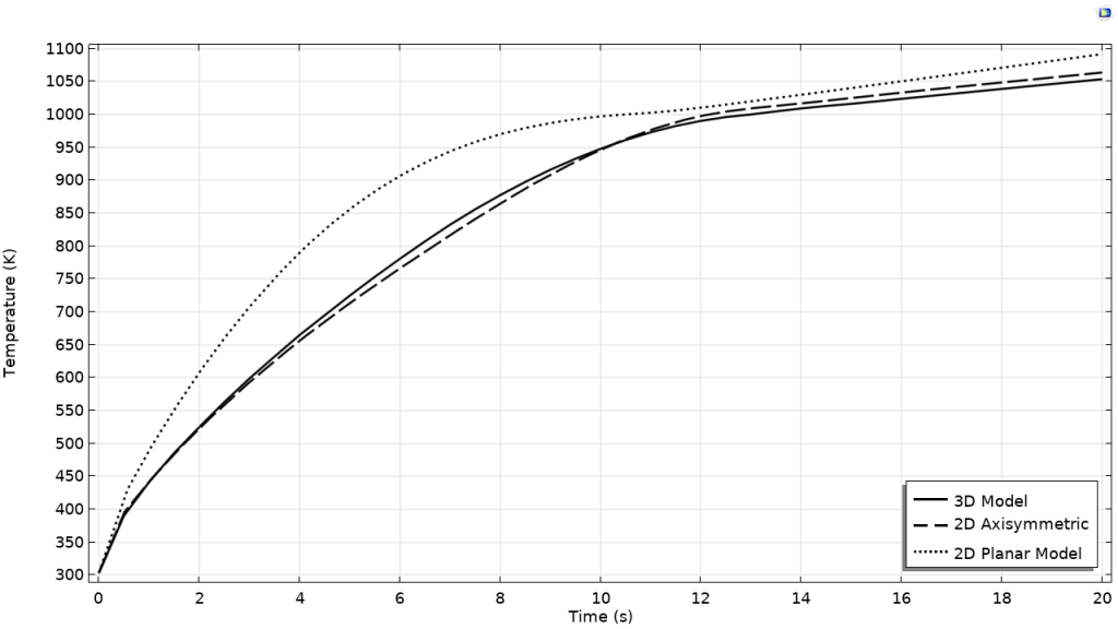 Comparison of the two-dimensional and three-dimensional model results.
The importance of building 2D models cannot be overemphasized, as they can often provide a very good estimate of the 3D solution, and it is much easier to investigate meshing, solver, and discretization strategies. As you expand these types of models, you will likely also want to include more physics, such as solving for the mechanical properties: Induction Hardening of a Cylindrical Pin.
Closing Remarks
We have shown here that it is easy to use the \mathbf{H}-field formulation to set up and solve induction heating of materials that are nonlinear with both magnetic field and temperature. This formulation can be more stable, and hence, converge faster than other approaches, particularly when you have strong nonlinearities.
Interested in getting started in this area? Download the tutorial model from the link below.


Comments (0)