

When we use conductive materials to move current, we often seek to minimize electrical resistance, but resistance and its effects — such as light and heat — can also be useful. Induction heating uses current to deliberately cause electrical behavior that heats up a material through resistance effects. These effects can be used for everything from melting iron at temperatures exceeding 1500°C to making a pot of tea on an induction stove!
Induction Creates Current Without Contact
As noted above, current flowing though a conductive material will generate heat due to electrical resistance. Toasters, hair dryers, room heaters, and other everyday devices make use of this effect. In these cases, the phenomenon is known as Joule heating or resistive heating. It occurs through direct physical contact between a conductive element and a current source.
By contrast, induction heating electrically heats up an object without direct physical contact with a current source. Instead, the conductive object (or workpiece) is placed near an induction coil, which carries alternating current (AC). The AC generates a time-varying magnetic field surrounding the induction coil. This field induces eddy currents that generate heat inside the workpiece.
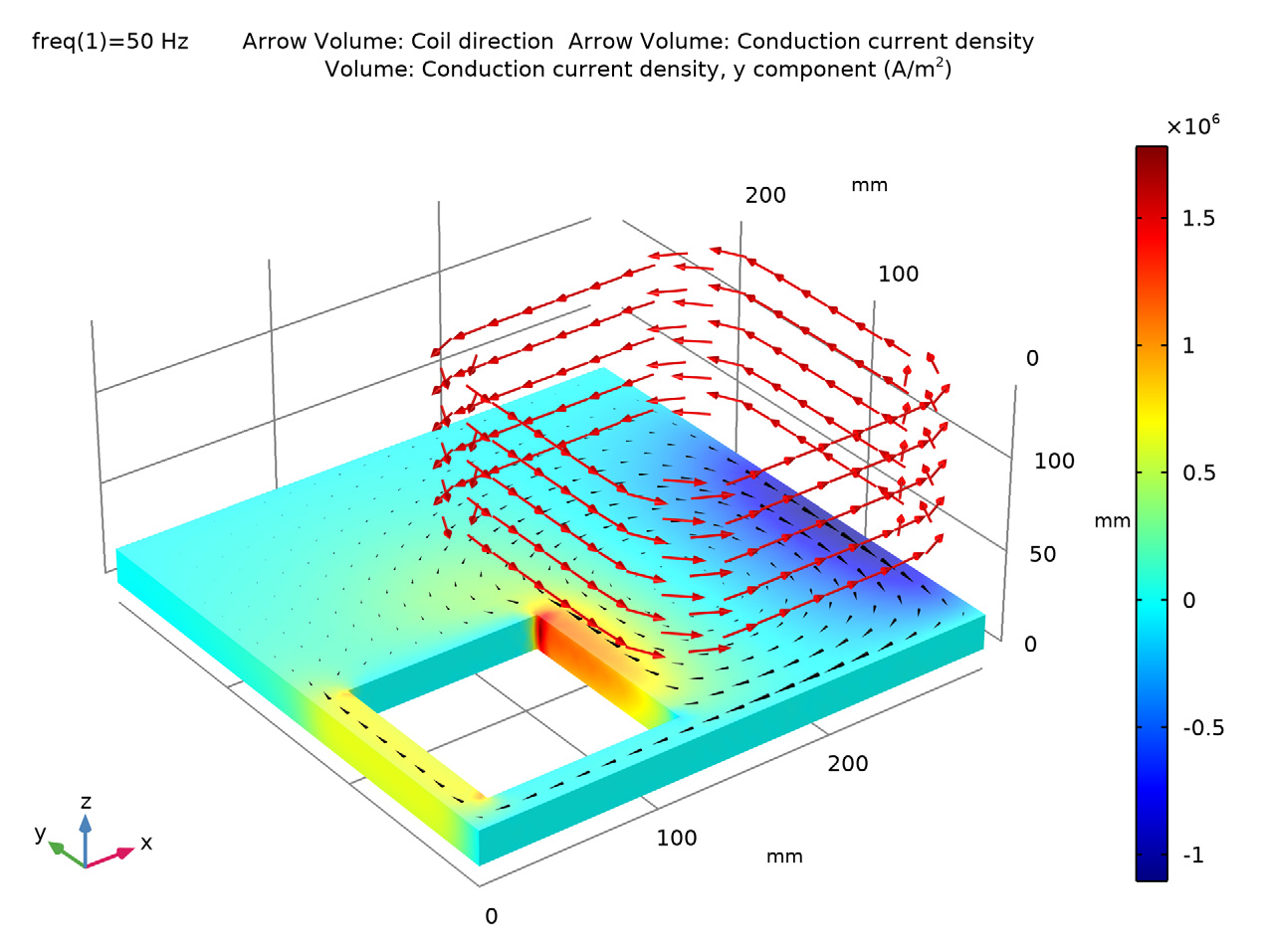
A simulation of current density induced in an aluminum conductor by a wound copper coil carrying a sinusoidally varying current. (Learn how to simulate this type of system here.)
To achieve useful inductive heating, a number of conditions must be met. The workpiece must be made from a material with high electrical conductivity. The applied current should cycle at a frequency that couples well with the conductivity and magnetic properties of the workpiece. Through careful selection of materials and frequency, we can inductively heat a ferrous workpiece from ambient temperature to more than 700°C in a matter of seconds. This occurs as the high permeability of iron-containing materials leads to stronger eddy currents and skin effects, in which alternating current flows more intensely around the surface of the workpiece. Inductive heating in ferrous metal is further intensified by the cyclical magnetization of iron crystals by alternating current flows. The rapidly shifting AC magnetic field leads to hysteresis losses, which generate still more heat.
What Are the Benefits of Induction Heating?
The ability to heat conductive materials efficiently and precisely — without touching them — makes induction heating an important aspect of many useful processes. For example, consider an induction stove. AC moving through an induction coil, which is hidden beneath the surface of the cooktop, creates an alternating magnetic field in an iron pot. Resistance effects in the pot generate enough heat to boil water, yet the cooktop and bottom of the pot are barely warmer than room temperature. This targeted heating is both safer and more efficient than typical stovetop cooking methods.
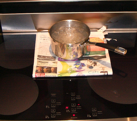
An induction stovetop heats a pot of water to a boil, yet the surface isn’t hot enough to ignite a newspaper under the pot. Image licensed under CC BY-SA 3.0, via Wikimedia Commons.
The benefits of induction heating are commensurately greater when applied on an industrial scale. Compared to other methods of heating and melting, induction furnaces consume less energy and emit less pollution. The cleanliness of induction heating also makes it an essential process for manufacturing semiconductors and other electronics.
Between the extremes of brewing tea and melting metals, induction heating can serve other purposes as well. Familiar metallurgical techniques like soldering, welding, and brazing can all be performed inductively. The heat of an induced current can also serve to harden a ferrous metal in a carefully controlled way, as demonstrated by the tutorial model described below…
A Model of Induction Effects in Ferrous Metal
Metalworking is a signature skill of civilization, as we acknowledge when we speak of the historical Bronze Age and Iron Age. Our own industrialized era effectively began with great advances in the production and processing of iron in the 19th century. Whereas metalsmiths traditionally hammered hot iron on an anvil, one small piece at a time, coal-fired mills could purify and harden unprecedented quantities of ferrous metal. Electrical metal processing advances in the 20th century included the development of induction hardening processes, a simulated example of which is shown below.
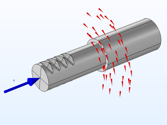
A process for induction hardening of a ferrous metal part by moving it through an induction coil. Current flow in the coil is shown in red.
This example models a process in which a ferrous workpiece is moved through an induction coil, which generates a field that induces heating in the part. This process is often used to harden drive shafts, mounting pins, and other similarly proportioned components that are subject to intense mechanical stresses. The model takes advantage of functionality in the AC/DC Module to account for coupled electromagnetic and heat transfer behaviors in the workpiece and physical changes that may result.
The AC/DC Module offers support for analyzing magnetic behaviors with user-selected constitutive relation options. The Effective B-H Curve option is well-suited for this analysis, as it takes into account both magnetic saturation (the point beyond which a material’s magnetization cannot be increased by an external field) and the Curie point of the workpiece material. When heated beyond the Curie point (named for Pierre Curie, who discovered and described it), a material will lose the magnetic properties that it displays at lower temperatures. Both saturation and Curie point effects will change the relationship between applied current and resulting changes in the workpiece.
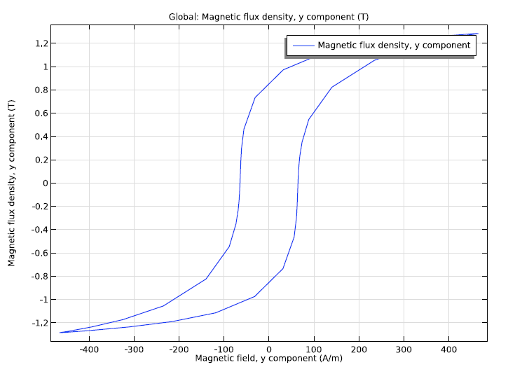
A graph of the B-H curve relationship, showing hysteretic behavior by plotting the magnetic flux density as a function of the magnetic field during one AC cycle. This graph is from an electromagnetics tutorial model, which can be used to reproduce the Testing Electromagnetic Analysis Method (TEAM) problem 32. The TEAM problem 32 evaluates numerical methods for the simulation of anisotropic magnetic hysteresis.
As this induction hardening process relies on the movement of the workpiece through the induction coil, the simulation must also account for displacement. This is addressed with a moving mesh via the Rotating Machinery, Magnetic interface using mixed vector and scalar potentials. The mesh must also account for skin effects, in which induced magnetic behavior varies between the surface and core of the workpiece.
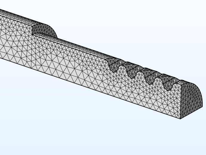
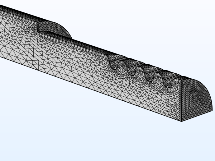
Mesh for two use cases in the induction hardening tutorial model: 1 kHz (left) and 25 kHz (right) AC frequencies.
Simulation Results for 2 Use Cases
While hardening metal with electrically induced heat is a useful effect, it is possible to have too much of a good thing. The same heat that hardens metal will also make it more brittle. To achieve the right balance of hardness and ductility in every region of the finished part, you can adjust key parameters of the induction hardening process. The results below can be used to compare two use cases that analyze the effects of three varying parameters:
- AC frequency
- External current level
- Velocity at which the workpiece is moved through the coil
")
")
A comparison of maximum temperature reached inside the workpiece in response to two different AC frequencies: 1 kHz (left) and 25 kHz (right).
Displacement and temperature change of a mechanical joint passing through an induction heating coil at f = 25 kHz, v = 10 mm/s.
As shown by the results, changing the coil’s AC frequency doesn’t just change the peak temperature, it also reshapes the distribution of induced heat throughout the workpiece. The resulting temperature field map can inform further analysis of metallurgical effects. For example, you can use simulated temperature data to predict metallurgical phase transition, by using the Metal Processing Module.
Try It Yourself
Try simulating electromagnetic induction heating effects in a metal component by downloading the tutorial model from the Application Gallery:


Comments (3)
Indrasis Mitra
December 7, 2021Hi Alan,
Excellent blog.
I though have an unrelated query. Is it possible to switch boundary condition in COMSOL in a periodic nature. Basically, I would like the inlet and outlet of a model to be interchanged during each half-cycle of a reciprocating flow, which contiues for a finite time.
Alan Petrillo
December 7, 2021 COMSOL EmployeeHi Indrasis, thank you for reading! The best way to get help with your modeling question would be to contact our Support team at http://www.comsol.com/support.
zack ivs
May 8, 2023I would like to ask a question in a simulation of induction welding of two 1 mm thick copper tubes using coils. Despite a magnetic flux density (phi) of 20e6A/m² and surface intégration on the 2D axes symmetric, the volumetric power density in the simulation is low (0.0019 W). Can anyone help me understand the reasons for this low power density and examine the simulation results and the freq=50hz? Thank you.